Chapter 5 Simpson-Paradox
5.1 Binomial-, Normal- und Gleichverteilte Werte in Antworten
\(X_b\) sei eine diskrete Variable, welche n=500 Zufallswerte mit dem Erwartungswert 2 und einem Wertebereich von 0 bis 4 aufweist:
\[ X_b = \mathcal{B}(k|p,n) ; k \in (0,1,2,3,4); p=0.5; n=500\] \(X_n\) sei eine stetige Variable, welche n=500 Zufallswerte mit dem Erwartungswert \(\mu\)=3 und einer Varianz \(\sigma^2\)=0.9 aufweist:
\[ X_n = \mathcal{N} (\mu,\sigma^2,n) \] wobei \(-\infty<x<\infty\), n=500, \(\mu\)=3 und \(\sigma^2\)=0.9.
\(X_u\) sei eine diskrete gleichverteilte Variable, welche n=500 Zufallswerte mit einem Wertebereich von 0 bis 4 aufweist:
\[X_u \in (0,1,2,3,4)\] wobei: \(P(X=x_i) = \frac{1}{5}\) wobei \(i \in (0,1,2,3,4)\)
set.seed(1896)
n <- 500 # Festlegung der Größe des Samples

#x <- round((1 + rnorm(n) + B),0)
xb = rbinom(n,4,0.5) # Binomialverteilte Werte
xn = rnorm(n,3,0.9) # Normalverteilte Werte
xu = runif(n,0,4) # Gleichverteilte Werte (uniform)

par(mfrow=c(1,3))
hist (xb)
hist (xn)
hist (xu)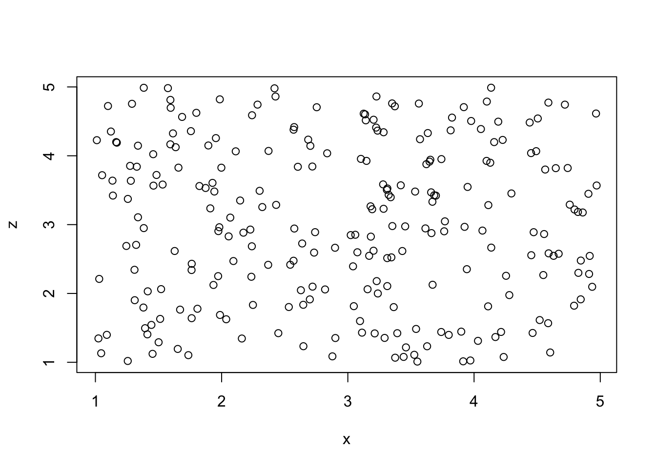
#ks.test (xn,"pnorm")
shapiro.test(xb)
##
## Shapiro-Wilk normality test
##
## data: xb
## W = 0.90804, p-value < 2.2e-16shapiro.test(xn)##
## Shapiro-Wilk normality test
##
## data: xn
## W = 0.99616, p-value = 0.2701shapiro.test(xu)##
## Shapiro-Wilk normality test
##
## data: xu
## W = 0.95606, p-value = 4.755e-11yb = rbinom(n,4,0.5) # Binomialverteilte Werte
yn = rnorm(n,3,0.9) # Normalverteilte Werte
yu = runif(n,0,4) # Gleichverteilte Werte (uniform)
par(mfrow=c(1,3))
plot (xb,yb)
plot (xn,yn)
plot (xu,yu)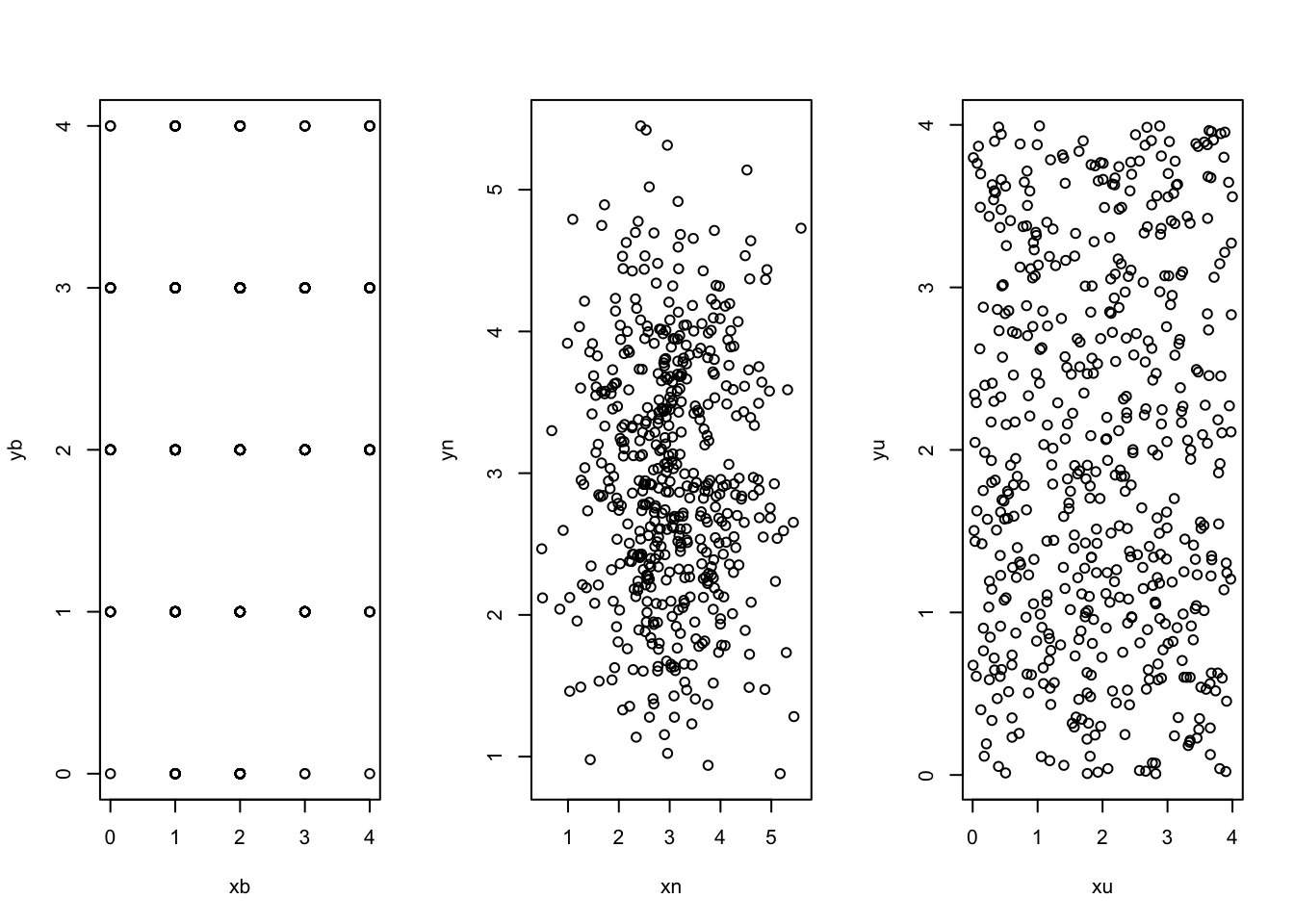
5.2 Example with typical individualistic Response-Patter
Befragte unterscheiden sich bei Einsatz von Skalen als Bewertungsinstrument, z.B. in Bevorzugung der Skalenmitte oder der Skalenextreme (Schwartz (2006)). Individualistisch orientierte Befragte tendieren zu letzterem. Im folgenden wird eine Stichprobe erzeugt, in welcher eine solche Tendenz durch die Zufallsvariable \(B\) (Bewertungs-Bias) einbezogen wird.
Dies führt dazu, dass eine tendenziell zweigipflige Häufigkeitsverteilung resultiert, die umso ausgeprägter ist, je stärker die Tendenz zu Extremen ausgeprägt ist.
\(X\) wird hier als stetige normalverteilte Zufallsvariable dargestellt.
set.seed(1896)
n <- 500 # Festlegung der Größe des Samples

B=rnorm(n)
B=ifelse (B<0, 2,4)
hist (B)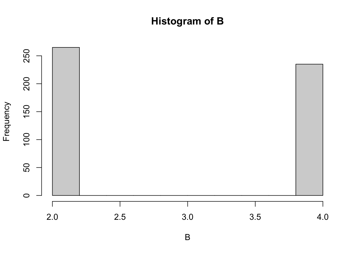
x = (1*B + rnorm(n))/1.5+1

hist (x)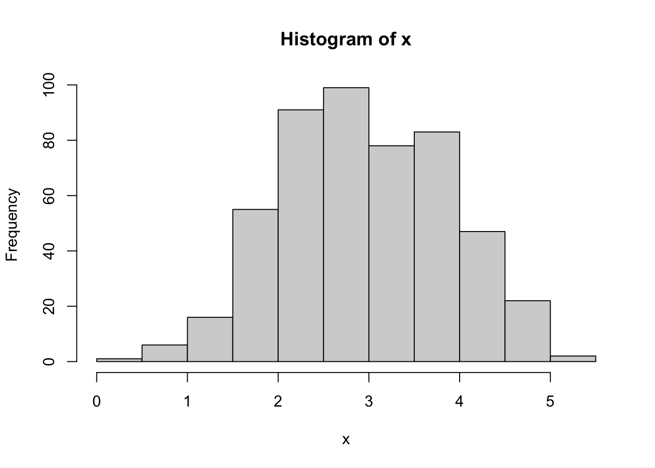
Da es sich bei dieser Tendenz um ein bevorzugtes Antwortmuster handelt, wird diese Präferenz auch in der abhängigen Variable berücksichtigt.
Auch hier ist eine Tendenz zu zwei Gipfeln enthalten, was in der Darstellung jedoch verdeckt bleibt.
Die Variable \(Y\) ergibt sich als Ergebnis des Bewertungs-Bias (\(B\)), eines normalverteilten Zufallswertes und dem Wert \(X\), wobei ein negativer Zusammenhang zwischen \(X\) und \(Y\) determiniert wird.
\[y_i = 1.5 \cdot B + \mathcal{N(0,1)} - 1.0 \cdot x_i) \]
y <-  (1.5*B + rnorm(n) - x)

#y <- ifelse (y<1,1,y)
#y <- ifelse (y>5,5,y)

hist (y)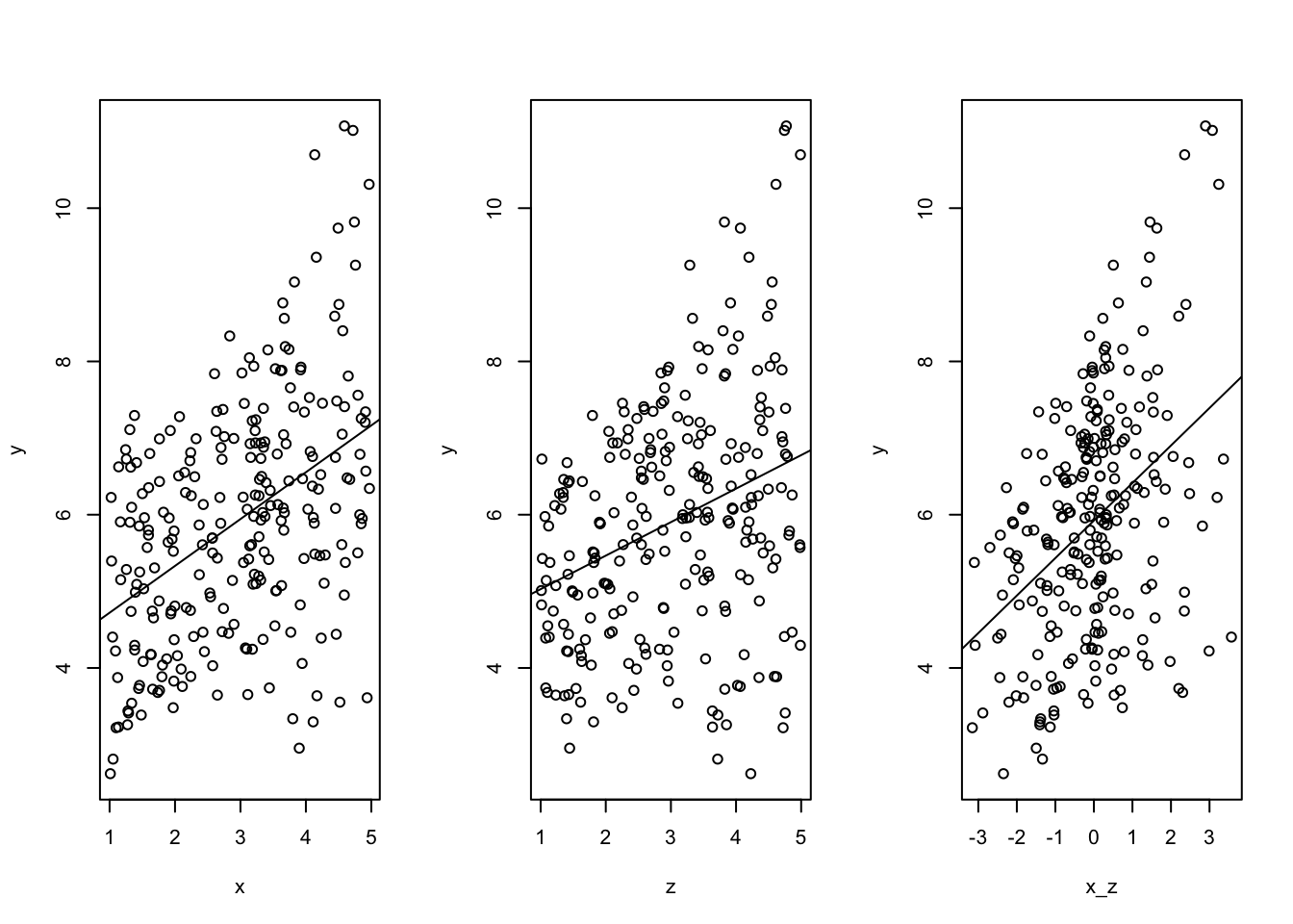
shapiro.test(y)##
## Shapiro-Wilk normality test
##
## data: y
## W = 0.99577, p-value = 0.1979plot ((x),y)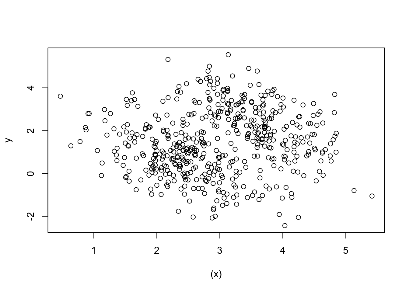
summary (lm(y~x)) ##
## Call:
## lm(formula = y ~ x)
##
## Residuals:
## Min 1Q Median 3Q Max
## -4.0085 -1.0183 -0.0384 1.0819 4.0678
##
## Coefficients:
## Estimate Std. Error t value Pr(>|t|)
## (Intercept) 1.13056 0.22763 4.967 9.38e-07 ***
## x 0.11028 0.07353 1.500 0.134
## ---
## Signif. codes: 0 '***' 0.001 '**' 0.01 '*' 0.05 '.' 0.1 ' ' 1
##
## Residual standard error: 1.493 on 498 degrees of freedom
## Multiple R-squared: 0.004496, Adjusted R-squared: 0.002497
## F-statistic: 2.249 on 1 and 498 DF, p-value: 0.1343summary (lm(y~x+B)) ##
## Call:
## lm(formula = y ~ x + B)
##
## Residuals:
## Min 1Q Median 3Q Max
## -2.87227 -0.69241 -0.04658 0.68645 2.72531
##
## Coefficients:
## Estimate Std. Error t value Pr(>|t|)
## (Intercept) -0.005326 0.154789 -0.034 0.973
## x -1.032843 0.065119 -15.861 <2e-16 ***
## B 1.537044 0.059223 25.953 <2e-16 ***
## ---
## Signif. codes: 0 '***' 0.001 '**' 0.01 '*' 0.05 '.' 0.1 ' ' 1
##
## Residual standard error: 0.9736 on 497 degrees of freedom
## Multiple R-squared: 0.5773, Adjusted R-squared: 0.5756
## F-statistic: 339.4 on 2 and 497 DF, p-value: < 2.2e-16Eine Regressionsanalyse weist auf einen falsch positiven Zusammenhang zwischen \(X\) und \(Y\) hin. Wird der Bewerter-Bias (\(B\)) als “gemeinsame Ursache” einbezogen, wird auch der Zusammenhang zwischen \(X\) und \(Y\) richtig geschätzt.
data <- data.frame(cbind(B,x,y))

subdata1 <-subset(data,B==2)
subdata2 <-subset(data,B==4)

summary (lm(subdata1$y~subdata1$x))
##
## Call:
## lm(formula = subdata1$y ~ subdata1$x)
##
## Residuals:
## Min 1Q Median 3Q Max
## -2.45050 -0.69987 0.02945 0.68090 2.73421
##
## Coefficients:
## Estimate Std. Error t value Pr(>|t|)
## (Intercept) 2.96380 0.21576 13.74 <2e-16 ***
## subdata1$x -0.98876 0.08706 -11.36 <2e-16 ***
## ---
## Signif. codes: 0 '***' 0.001 '**' 0.01 '*' 0.05 '.' 0.1 ' ' 1
##
## Residual standard error: 0.9738 on 263 degrees of freedom
## Multiple R-squared: 0.3291, Adjusted R-squared: 0.3265
## F-statistic: 129 on 1 and 263 DF, p-value: < 2.2e-16summary (lm(subdata2$y~subdata2$x)) ##
## Call:
## lm(formula = subdata2$y ~ subdata2$x)
##
## Residuals:
## Min 1Q Median 3Q Max
## -2.86538 -0.70170 -0.09087 0.74500 2.61145
##
## Coefficients:
## Estimate Std. Error t value Pr(>|t|)
## (Intercept) 6.3452 0.3603 17.61 <2e-16 ***
## subdata2$x -1.0889 0.0982 -11.09 <2e-16 ***
## ---
## Signif. codes: 0 '***' 0.001 '**' 0.01 '*' 0.05 '.' 0.1 ' ' 1
##
## Residual standard error: 0.9743 on 233 degrees of freedom
## Multiple R-squared: 0.3454, Adjusted R-squared: 0.3426
## F-statistic: 122.9 on 1 and 233 DF, p-value: < 2.2e-16Wird die Stichprobe unterteilt in links- vs. rechts-tendierender Antworten, werden in beiden Teilstichproben der “richtige” negative Zusammenhang geschätzt. In realen Daten ist dieses Wissen jedoch primär nicht vorhanden.
5.2.1 Skalenkorrektur im Gesamtsample
Die von Schwartz (2006) vorgeschlagene Skalenkorrektur scheint in diesem Beispiel nur bedingt sinnvoll, da ja nur zwei Wertungen vorliegen. Beim Vorliegen von mehr Aussagen, gewinnt die “Extraktion” der Antworttendenz an Präzision. Dennoch wird der Steigungskoeffizient richtig bestimmt.
data <- data.frame(cbind(B,x,y))

# individual-wise scale correction
data$x_c <- x-((x+y)/2)
data$y_c <- y-((x+y)/2)

hist (data$x_c)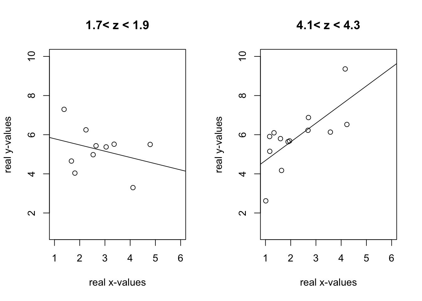
plot (data$x_c,data$y_c)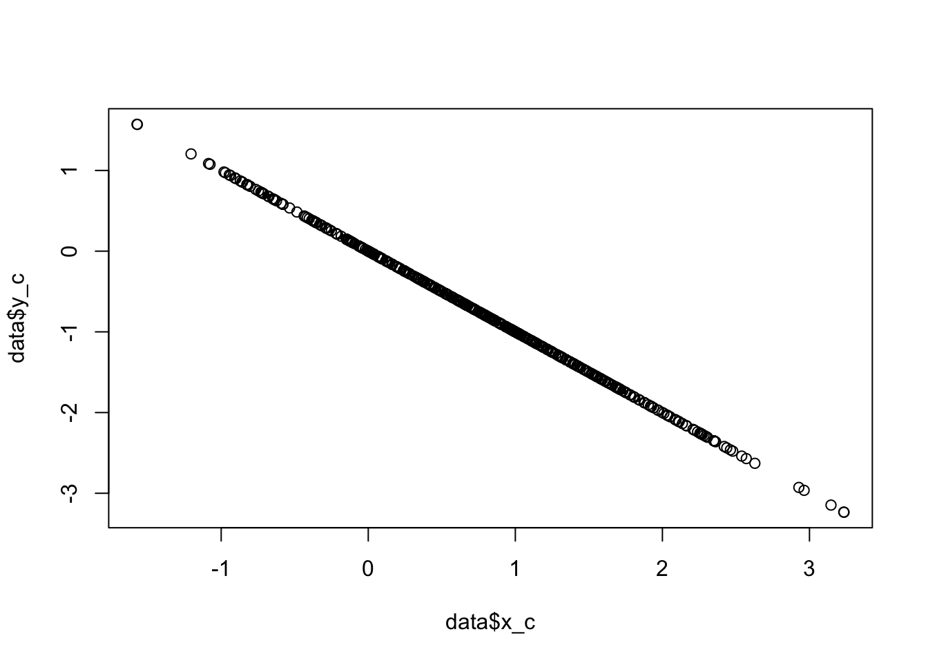
summary (lm(data$y_c~data$x_c)) ## Warning in summary.lm(lm(data$y_c ~ data$x_c)): essentially perfect fit: summary
## may be unreliable##
## Call:
## lm(formula = data$y_c ~ data$x_c)
##
## Residuals:
## Min 1Q Median 3Q Max
## -8.942e-16 -5.940e-17 -3.780e-17 -1.120e-17 1.749e-14
##
## Coefficients:
## Estimate Std. Error t value Pr(>|t|)
## (Intercept) -6.355e-16 4.725e-17 -1.345e+01 <2e-16 ***
## data$x_c -1.000e+00 4.173e-17 -2.397e+16 <2e-16 ***
## ---
## Signif. codes: 0 '***' 0.001 '**' 0.01 '*' 0.05 '.' 0.1 ' ' 1
##
## Residual standard error: 7.906e-16 on 498 degrees of freedom
## Multiple R-squared: 1, Adjusted R-squared: 1
## F-statistic: 5.743e+32 on 1 and 498 DF, p-value: < 2.2e-16summary (lm(data$y_c~data$x_c+data$B)) ## Warning in summary.lm(lm(data$y_c ~ data$x_c + data$B)): essentially perfect
## fit: summary may be unreliable##
## Call:
## lm(formula = data$y_c ~ data$x_c + data$B)
##
## Residuals:
## Min 1Q Median 3Q Max
## -9.292e-16 -7.850e-17 -3.000e-17 1.100e-18 1.745e-14
##
## Coefficients:
## Estimate Std. Error t value Pr(>|t|)
## (Intercept) -7.944e-16 1.206e-16 -6.585e+00 1.16e-10 ***
## data$x_c -1.000e+00 4.233e-17 -2.362e+16 < 2e-16 ***
## data$B 3.762e-17 3.593e-17 1.047e+00 0.296
## ---
## Signif. codes: 0 '***' 0.001 '**' 0.01 '*' 0.05 '.' 0.1 ' ' 1
##
## Residual standard error: 7.905e-16 on 497 degrees of freedom
## Multiple R-squared: 1, Adjusted R-squared: 1
## F-statistic: 2.872e+32 on 2 and 497 DF, p-value: < 2.2e-165.3 Intervallskalierte Daten
Im folgenden wird dargestellt, dass der Informationsverlust bei der Transformation der stetigen Daten in intervallskalierte Daten diesen Effekt möglicherweise verstärkt. Der negative Zusammenhang stellt sich hier als signifikant positiver Zusammenhang dar.
data <- data.frame(cbind(B,x,y))

# intervall-scaled values
data$x_i <- round(x,0)
#data$y_i <- round((y+4)/10*6,0)
data$y_i <- round(y,0)

hist (data$x_i)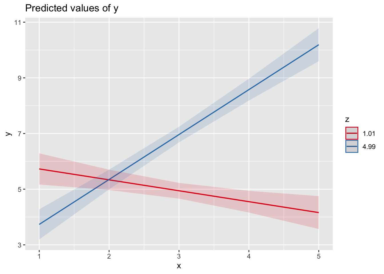
hist (data$y_i)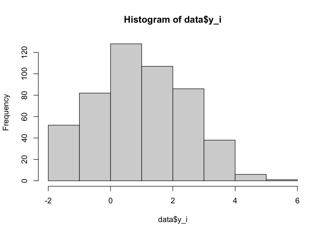
plot (data$x_i,data$y_i)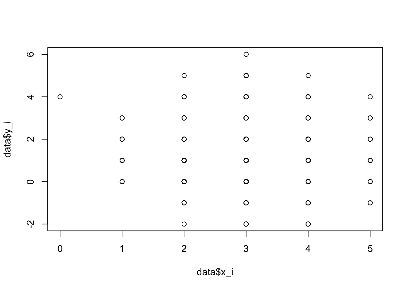
summary (lm(data$y_i~data$x_i)) ##
## Call:
## lm(formula = data$y_i ~ data$x_i)
##
## Residuals:
## Min 1Q Median 3Q Max
## -3.5965 -1.3198 -0.3198 1.4035 4.5419
##
## Coefficients:
## Estimate Std. Error t value Pr(>|t|)
## (Intercept) 1.0432 0.2180 4.784 2.27e-06 ***
## data$x_i 0.1383 0.0698 1.982 0.0481 *
## ---
## Signif. codes: 0 '***' 0.001 '**' 0.01 '*' 0.05 '.' 0.1 ' ' 1
##
## Residual standard error: 1.511 on 498 degrees of freedom
## Multiple R-squared: 0.007823, Adjusted R-squared: 0.005831
## F-statistic: 3.926 on 1 and 498 DF, p-value: 0.04808summary (lm(data$y_i~data$x_i+data$B)) ##
## Call:
## lm(formula = data$y_i ~ data$x_i + data$B)
##
## Residuals:
## Min 1Q Median 3Q Max
## -3.11703 -0.91469 0.02325 0.88297 3.08531
##
## Coefficients:
## Estimate Std. Error t value Pr(>|t|)
## (Intercept) -0.28766 0.16086 -1.788 0.0743 .
## data$x_i -0.85972 0.06431 -13.367 <2e-16 ***
## data$B 1.46089 0.06237 23.422 <2e-16 ***
## ---
## Signif. codes: 0 '***' 0.001 '**' 0.01 '*' 0.05 '.' 0.1 ' ' 1
##
## Residual standard error: 1.043 on 497 degrees of freedom
## Multiple R-squared: 0.5284, Adjusted R-squared: 0.5265
## F-statistic: 278.4 on 2 and 497 DF, p-value: < 2.2e-16Auch hier scheint die Skalenkorrektur hilfreich, um den richtigen Zusammenhang zwischen \(X\) und \(Y\) zu bestimmen, ohne diesen Einfluss zu kennen.
# individual-wise scale correction
data$x_ic <- data$x_i-((data$x_i+data$y_i)/2)
data$y_ic <- data$y_i-((data$x_i+data$y_i)/2)

hist (data$x_ic)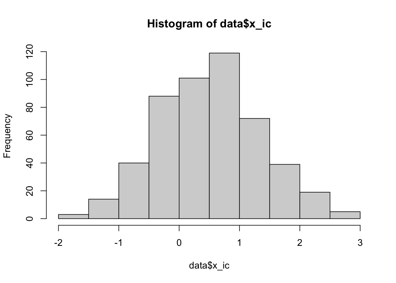
plot (data$x_ic,data$y_ic)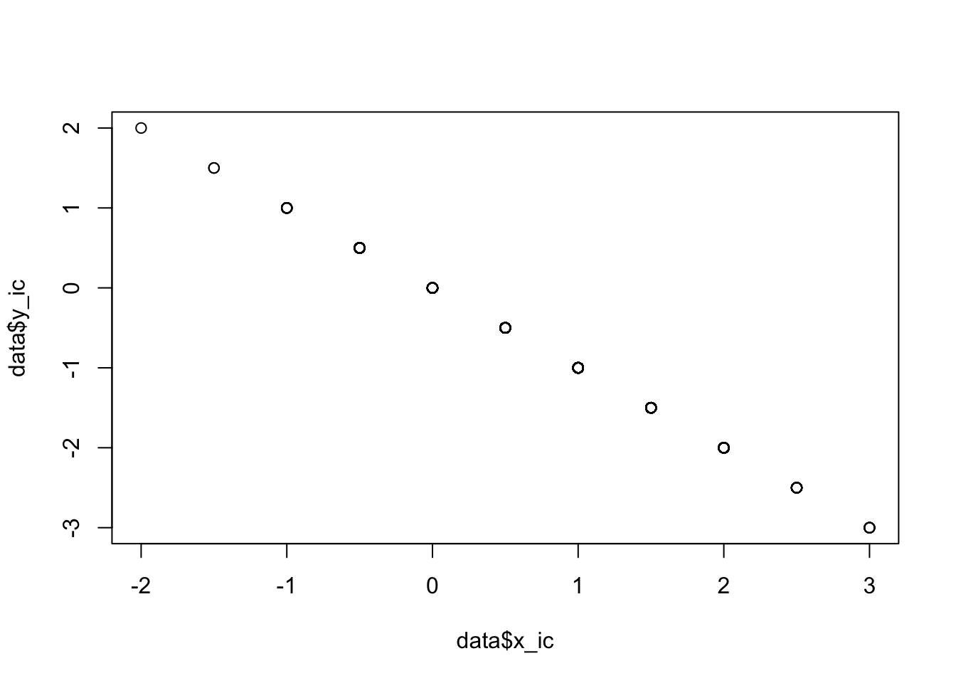
summary (lm(data$y_ic~data$x_ic)) ##
## Call:
## lm(formula = data$y_ic ~ data$x_ic)
##
## Residuals:
## Min 1Q Median 3Q Max
## -1.569e-15 -7.390e-17 -6.060e-17 -2.800e-17 3.116e-14
##
## Coefficients:
## Estimate Std. Error t value Pr(>|t|)
## (Intercept) 1.112e-15 8.337e-17 1.334e+01 <2e-16 ***
## data$x_ic -1.000e+00 7.264e-17 -1.377e+16 <2e-16 ***
## ---
## Signif. codes: 0 '***' 0.001 '**' 0.01 '*' 0.05 '.' 0.1 ' ' 1
##
## Residual standard error: 1.4e-15 on 498 degrees of freedom
## Multiple R-squared: 1, Adjusted R-squared: 1
## F-statistic: 1.895e+32 on 1 and 498 DF, p-value: < 2.2e-16summary (lm(data$y_ic~data$x_ic+data$B)) ##
## Call:
## lm(formula = data$y_ic ~ data$x_ic + data$B)
##
## Residuals:
## Min 1Q Median 3Q Max
## -1.631e-15 -1.222e-16 -3.020e-17 -7.000e-19 3.110e-14
##
## Coefficients:
## Estimate Std. Error t value Pr(>|t|)
## (Intercept) 9.533e-16 2.122e-16 4.491e+00 8.81e-06 ***
## data$x_ic -1.000e+00 7.353e-17 -1.360e+16 < 2e-16 ***
## data$B 6.073e-17 6.347e-17 9.570e-01 0.339
## ---
## Signif. codes: 0 '***' 0.001 '**' 0.01 '*' 0.05 '.' 0.1 ' ' 1
##
## Residual standard error: 1.4e-15 on 497 degrees of freedom
## Multiple R-squared: 1, Adjusted R-squared: 1
## F-statistic: 9.473e+31 on 2 and 497 DF, p-value: < 2.2e-165.4 Education - Salary
Im Beispiel wird der Simpsoneffekt aus dem Projektseminar überprüft. Der negative Effekt zwischen Education und Salary wird fälschlich als positiv dargestellt.
library(dplyr)##
## Attaching package: 'dplyr'## The following objects are masked from 'package:stats':
##
## filter, lag## The following objects are masked from 'package:base':
##
## intersect, setdiff, setequal, unionlibrary(scales)
set.seed(1899)
n = 1000
Management = rbinom(n, 2, 0.5)
Education = rnorm(n) + Management
Salary = Management * 2 + rnorm(n) - Education * 0.3
Salary = sample(1000:1100,1) + rescale(Salary, to = c(0, 10000))
Education = rescale(Education, to = c(0, 7))
data <- data.frame(Salary, Education, Management)
summary(lm(Salary~Education,data))##
## Call:
## lm(formula = Salary ~ Education, data = data)
##
## Residuals:
## Min 1Q Median 3Q Max
## -6042.2 -1100.3 -15.4 1143.1 4491.3
##
## Coefficients:
## Estimate Std. Error t value Pr(>|t|)
## (Intercept) 4978.04 136.08 36.58 <2e-16 ***
## Education 440.18 41.58 10.59 <2e-16 ***
## ---
## Signif. codes: 0 '***' 0.001 '**' 0.01 '*' 0.05 '.' 0.1 ' ' 1
##
## Residual standard error: 1622 on 998 degrees of freedom
## Multiple R-squared: 0.1009, Adjusted R-squared: 0.1
## F-statistic: 112.1 on 1 and 998 DF, p-value: < 2.2e-16Um den Wert für die Skalenkorrektur zu bestimmen, wird zuerst eine z-Transformation durchgeführt.
5.5 z-Transformation
data$sal_z = scale(data$Salary)
data$edu_z = scale(data$Education)
data$man_z = scale(data$Management)
summary(lm(sal_z~edu_z,data))
##
## Call:
## lm(formula = sal_z ~ edu_z, data = data)
##
## Residuals:
## Min 1Q Median 3Q Max
## -3.5338 -0.6435 -0.0090 0.6685 2.6267
##
## Coefficients:
## Estimate Std. Error t value Pr(>|t|)
## (Intercept) -9.013e-17 3.000e-02 0.00 1
## edu_z 3.177e-01 3.001e-02 10.59 <2e-16 ***
## ---
## Signif. codes: 0 '***' 0.001 '**' 0.01 '*' 0.05 '.' 0.1 ' ' 1
##
## Residual standard error: 0.9487 on 998 degrees of freedom
## Multiple R-squared: 0.1009, Adjusted R-squared: 0.1
## F-statistic: 112.1 on 1 and 998 DF, p-value: < 2.2e-16Die z-Transformation allein bringt keinen Vorteil. Es wird nach wie vor ein falsch positiver Zusammenhang dargestellt.
5.6 Skalenkorrektur
data$sal_corr = data$sal_z -(( data$sal_z+data$edu_z+data$man_z)/3)
data$edu_corr = data$edu_z -(( data$sal_z+data$edu_z+data$man_z)/3)
data$man_corr = data$man_z -(( data$sal_z+data$edu_z+data$man_z)/3)
summary(lm(sal_corr~edu_corr,data))
##
## Call:
## lm(formula = sal_corr ~ edu_corr, data = data)
##
## Residuals:
## Min 1Q Median 3Q Max
## -1.21962 -0.19715 -0.00556 0.20658 1.00664
##
## Coefficients:
## Estimate Std. Error t value Pr(>|t|)
## (Intercept) -5.546e-17 9.653e-03 0.00 1
## edu_corr -7.256e-01 1.478e-02 -49.09 <2e-16 ***
## ---
## Signif. codes: 0 '***' 0.001 '**' 0.01 '*' 0.05 '.' 0.1 ' ' 1
##
## Residual standard error: 0.3053 on 998 degrees of freedom
## Multiple R-squared: 0.7072, Adjusted R-squared: 0.7069
## F-statistic: 2410 on 1 and 998 DF, p-value: < 2.2e-16Die Skalenkorrektur funktioniert hier also auch im Kontext von unterschiedlich skalierten Daten. Es resultiert ein richtig - negativer Koeffizient.
5.7 NCA
Es wird die Frage untersucht, ob Education eine notwendige Bedingung für Salary ist.
plot (data$Education,data$Salary)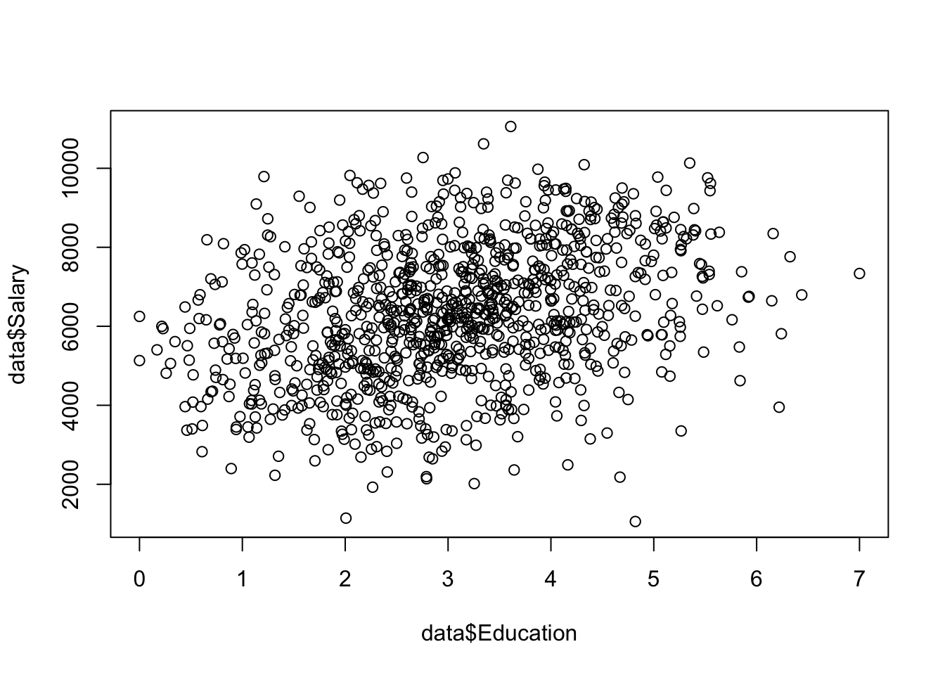 Der Plot verdeutlicht durch seine Wolkenform eine Tendenz zu Äquvalenz sowie simultan eine Tendenz zu Necessity oder Sufficiency.
Es ist also kein heterogenes Muster vorhanden, sondern (möglicherweise) mehrere heterogene, sich überlagernde Muster.
subdata <- subset(data,Management==1)

par(mfrow=c(1,2))
plot (subdata$Education,subdata$Salary)

maxvalue= max(subdata$Education)
plot (maxvalue-subdata$Education,subdata$Salary)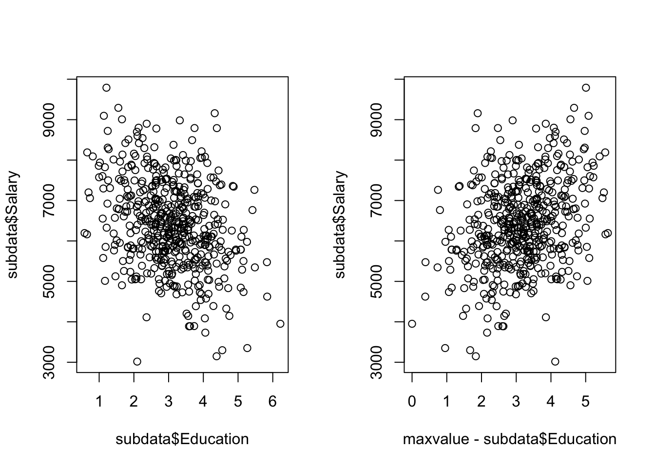
5.8 Interaktion
#normalverteilte Zufallswerte
set.seed(1896)
n <- 1000 # Festlegung der Größe des Samples

U1 = rnorm(n)

U2 = rnorm(n)

X = 1*U1 + 1*U2 + 0.75*(U1*U2) + 1*rnorm(n)

#Y = -1*U1 + (-1*U2) -0.7*(U1*U2)+1*rnorm(n)

Y= X - 2.5*U1 + rnorm(n)

par(mfrow=c(1,3))
plot(X,Y)
plot(U1,X)
plot(U2,X)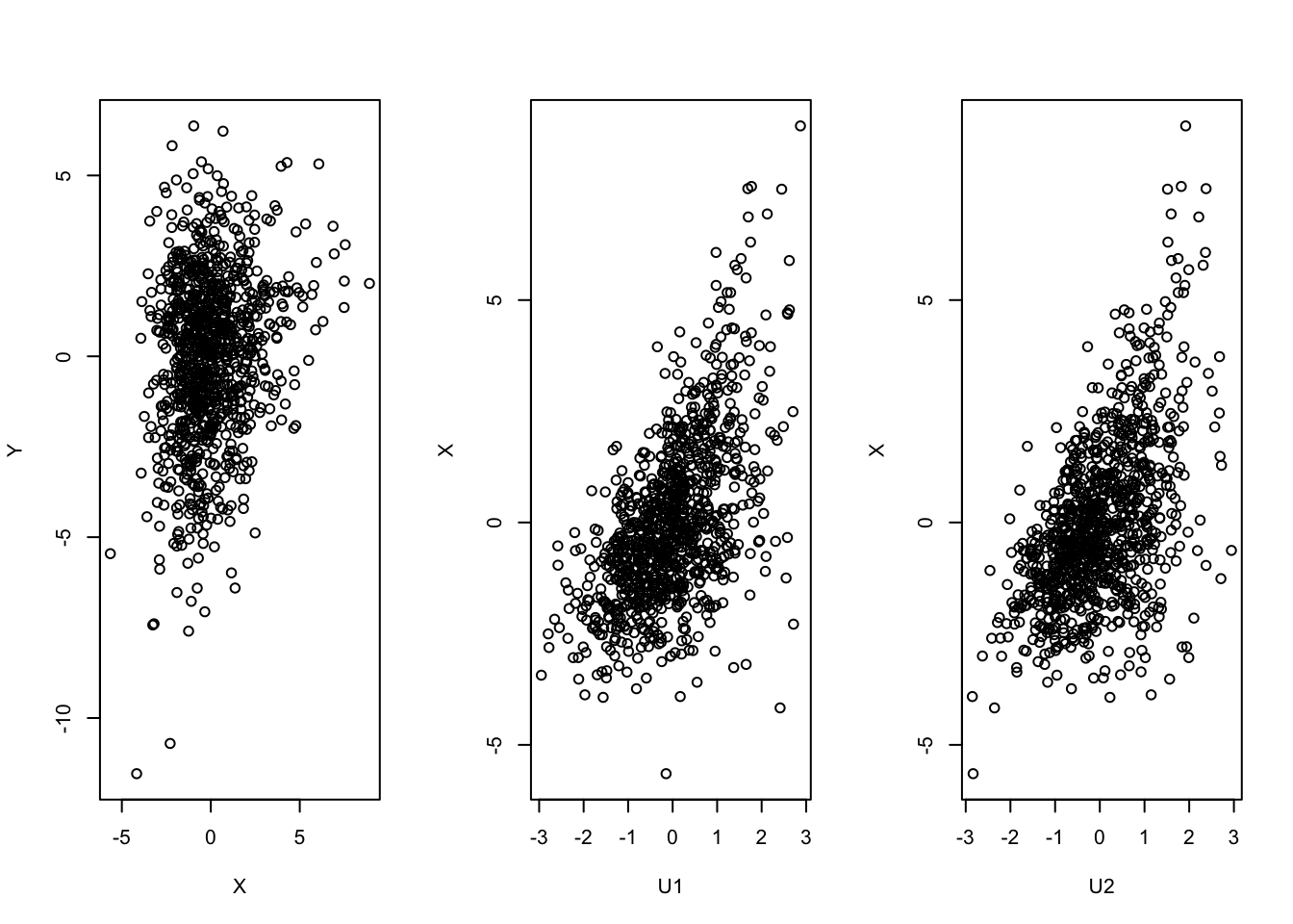
5.9 Gleichverteilte Zufallswerte
set.seed(1896)

 # erzeuge 3 Integer-Zahlen zwischen 1 und 5
 U <- floor(runif(100, min=1, max=6))
 X <- U + floor(runif(100, min=1, max=6))


 Y <- ifelse(U>3,0.5*X + 0.5*U,NA)

data <- data.frame(cbind(U,X,Y))

subdata <-subset(data,U>3)


#Z <- 1*X - 1*U
 #summary (lm(Y~X + Z))

par(mfrow=c(1,2))
plot(subdata$X,subdata$Y)
#plot(subdata$Z,subdata$Y)
plot(subdata$U,subdata$Y)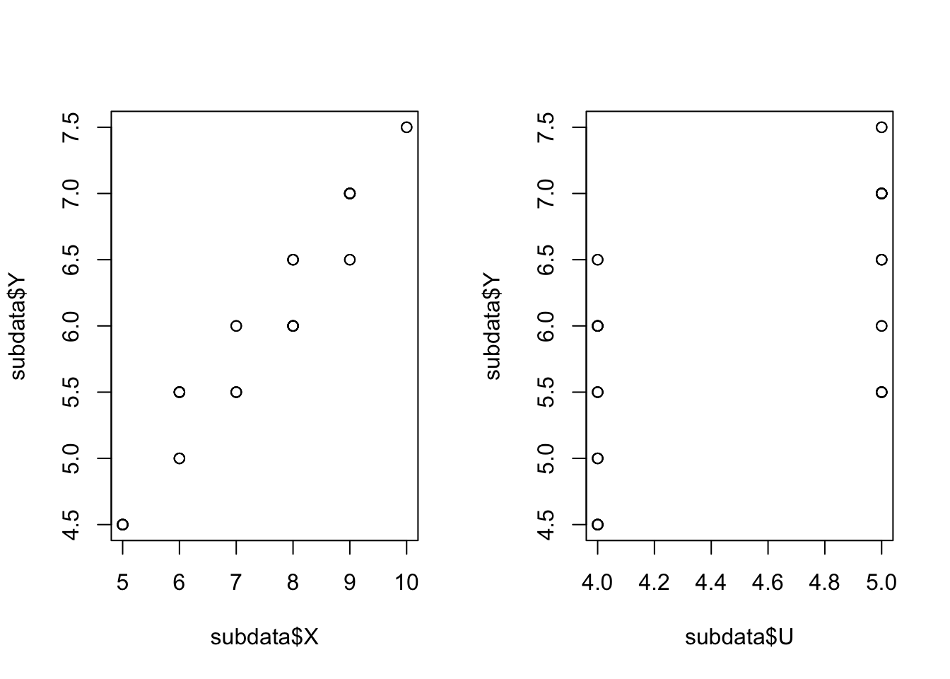
5.10 Real data example
In diesem Beispiel werden die Wahrscheinlichkeiten für die darwinistische und missionarische Identität mit der Wahrscheinlichkeit für die Wahrnehmung von Gemeinschaftssinn untersucht.
data <- read.csv2(file='data/User - User_Prov_Merge_v9 13.08.21_N539.csv',header=TRUE)
ncol(data)
## [1] 691Die folgenden Anpassungen entsprechen denen aus dem Projekt “Provider-User Fit”
5.11 NCA - Identität (Rohwerte) und SOC
subdata <- data[,c("x141", "x142","x143", "x144","x145","x146", "x228","x229","x231","x242","x238","x239", "x234","x235","x236", "x114")]

subdata <- subset(subdata,subdata$x114<2) # deutsches sample
#subdata <- subset(subdata,subdata$x114==2) # chinesisches sample

subdata <- subdata[complete.cases(subdata),]

subdata$mission = subdata$x141 + subdata$x142 + subdata$x143
subdata$darwin = subdata$x144 + subdata$x145 + subdata$x146
subdata$soc = subdata$x228 + subdata$x229 + subdata$x231

par(mfrow=c(1,3))
plot (subdata$darwin,subdata$mission)
plot (subdata$darwin,subdata$soc)
plot (subdata$mission,subdata$soc)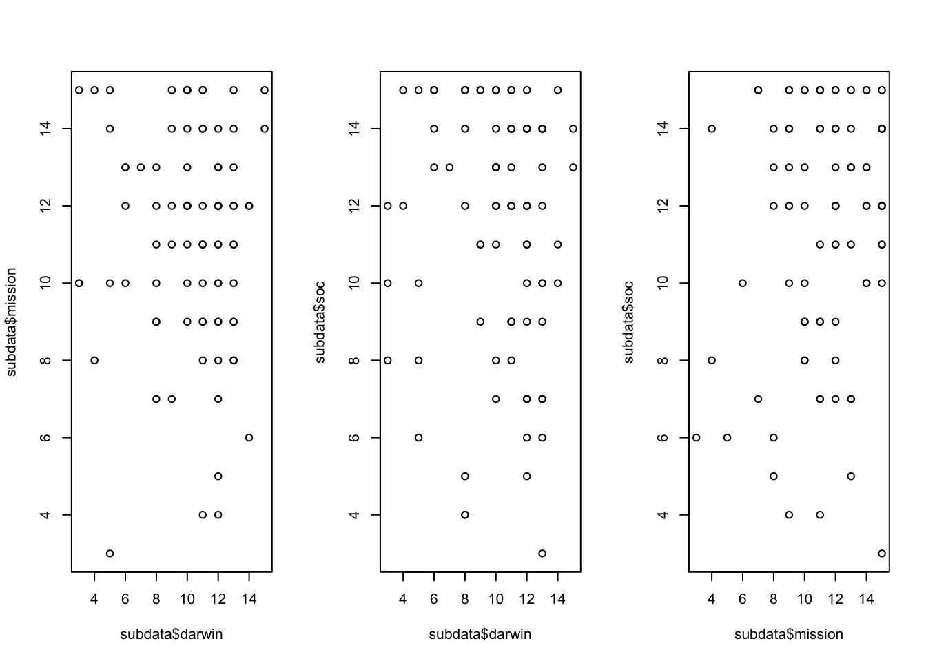
Die folgende Kalibrierung erfolg anhand theoretischer Ankerpunkte (semantische Skalenpunkte)
library(QCA)## Loading required package: admisc##
## Attaching package: 'admisc'## The following objects are masked from 'package:dplyr':
##
## compute, recode##
## To cite package QCA in publications, please use:
## Dusa, Adrian (2019) QCA with R. A Comprehensive Resource.
## Springer International Publishing.
##
## To run the graphical user interface, use: runGUI()a=1
b=3
c=5
subdata$x141_cbr <- calibrate(subdata$x141, type = "fuzzy",method ="direct", c(a,b,c))
subdata$x142_cbr <- calibrate(subdata$x142, type = "fuzzy",method ="direct", c(a,b,c))
subdata$x143_cbr <- calibrate(subdata$x143, type = "fuzzy",method ="direct", c(a,b,c))
subdata$x144_cbr <- calibrate(subdata$x144, type = "fuzzy",method ="direct", c(a,b,c))
subdata$x145_cbr <- calibrate(subdata$x145, type = "fuzzy",method ="direct", c(a,b,c))
subdata$x146_cbr <- calibrate(subdata$x146, type = "fuzzy",method ="direct", c(a,b,c))
subdata$x228_cbr <- calibrate(subdata$x228, type = "fuzzy",method ="direct", c(a,b,c))
subdata$x229_cbr <- calibrate(subdata$x229, type = "fuzzy",method ="direct", c(a,b,c))
subdata$x231_cbr <- calibrate(subdata$x231, type = "fuzzy",method ="direct", c(a,b,c))
subdata$p_mi <- subdata$x141_cbr*subdata$x142_cbr*subdata$x143_cbr
subdata$p_da <- subdata$x144_cbr*subdata$x145_cbr*subdata$x146_cbr
subdata$p_soc <- subdata$x228_cbr*subdata$x229_cbr*subdata$x231_cbr
par(mfrow=c(2,2))
plot (subdata$p_da,subdata$p_soc)
plot (subdata$p_mi,subdata$p_soc)
plot (subdata$p_da*subdata$p_mi,subdata$p_soc)
plot ((1-subdata$p_da)*(1-subdata$p_mi),subdata$p_soc)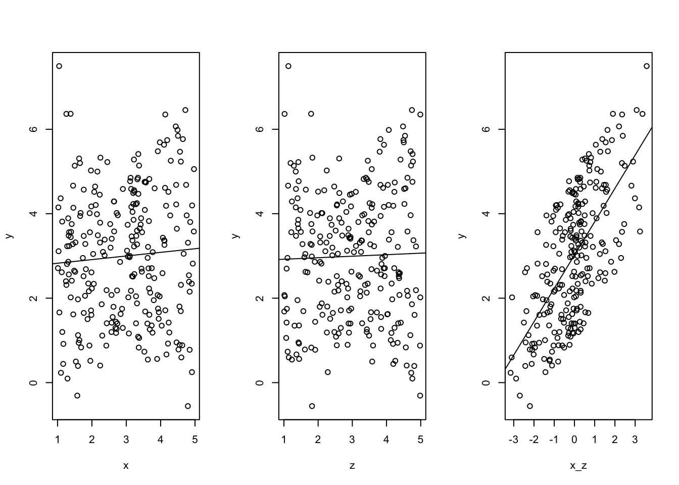 Die beiden unteren Abbildungen zeigen die Wahrscheinlichkeit einer undifferenzierten Identität (links), in der beide Indentitäten stark ausgeprägt sind, und unausgeprägten Identität (rechts), in der jede der beiden Identitäten unwahrscheinlich ist. Als Outcome wird der Gemeinschaftssinn abgebildet. Die Frage lautet also, ist die Wahrscheinliche Ausprägung einer, beider oder keiner der beiden eine (notwendige/ hinreichende) Bedingung für Gemeinschaftssinn.
Es folgt der Einbezug von Wettbewerb und Vertrauen. Die Frage lautet also: wie wahrscheinlich ist die hohe Ausprägung (Wahrnehmung, Bewertung) von Gemeinschaftssinn, wenn die Wahrscheinlichkeit für die darwinistische Identität hoch ist. Wie ändert sich dieses, wenn die Wahrscheinlichkeit des Darwinisten mit hoher Wahrscheinlichkeit für Wettbewerb oder Vertrauen einher geht.
Allein die Wahrscheinlichkeit einer darwinistischen Identität zeigt einen unsystematischen Zusammenhang mit der Wahrnehmung von Gemeinschaftssinn (oben links). Die Kombination Darwinisten mit Wettbewerb weist auf eine hinreichende Bedingung für Gemeinschaftssinn hin.
a=1
b=3
c=5

subdata$x242_cbr <- calibrate(subdata$x242, type = "fuzzy",method ="direct", c(a,b,c))
subdata$x238_cbr <- calibrate(subdata$x238, type = "fuzzy",method ="direct", c(a,b,c))
subdata$x239_cbr <- calibrate(subdata$x239, type = "fuzzy",method ="direct", c(a,b,c))

subdata$x234_cbr <- calibrate(subdata$x234, type = "fuzzy",method ="direct", c(a,b,c))
subdata$x235_cbr <- calibrate(subdata$x235, type = "fuzzy",method ="direct", c(a,b,c))
subdata$x236_cbr <- calibrate(subdata$x236, type = "fuzzy",method ="direct", c(a,b,c))

subdata$p_comp <- subdata$x242_cbr*subdata$x238_cbr*subdata$x239_cbr
subdata$p_tru <- subdata$x234_cbr*subdata$x235_cbr*subdata$x236_cbr

par(mfrow=c(3,3))

plot (subdata$p_da,subdata$p_soc, xlim=c(0,1), ylim=c(0,1))
plot (subdata$p_comp,subdata$p_soc, xlim=c(0,1),ylim=c(0,1))
plot (subdata$p_tru,subdata$p_soc, xlim=c(0,1),ylim=c(0,1))

plot (subdata$p_da*subdata$p_comp,subdata$p_soc, xlim=c(0,1),ylim=c(0,1))
plot (subdata$p_comp*subdata$p_tru,subdata$p_soc, xlim=c(0,1),ylim=c(0,1))
plot (subdata$p_da*subdata$p_tru,subdata$p_soc, xlim=c(0,1),ylim=c(0,1))

plot (subdata$p_da*subdata$p_comp*subdata$p_tru,subdata$p_soc, xlim=c(0,1),ylim=c(0,1))
Die Missionare nehmen Gemeinschaftssinn eher im Kontext von Vertrauen war.
par(mfrow=c(3,3))

plot (subdata$p_mi,subdata$p_soc, xlim=c(0,1), ylim=c(0,1))
plot (subdata$p_comp,subdata$p_soc, xlim=c(0,1),ylim=c(0,1))
plot (subdata$p_tru,subdata$p_soc, xlim=c(0,1),ylim=c(0,1))

plot (subdata$p_mi*subdata$p_comp,subdata$p_soc, xlim=c(0,1),ylim=c(0,1))
plot (subdata$p_comp*subdata$p_tru,subdata$p_soc, xlim=c(0,1),ylim=c(0,1))
plot (subdata$p_mi*subdata$p_tru,subdata$p_soc, xlim=c(0,1),ylim=c(0,1))

plot (subdata$p_mi*subdata$p_comp*subdata$p_tru,subdata$p_soc, xlim=c(0,1),ylim=c(0,1))
Im folgenden werden die Wahrscheinlichkeit eine darwinistische bzw. missionarische Identität anzugeben mit der Wahrscheinlichkeit, auch Gemeinschaftssinn wahrzunehmen dargestellt. Darwinisten stellt sich als notwendige Bedingung für die Bewertung von Gemeinschaftssinn mit Wettbewerb dar (oben rechts).
par(mfrow=c(2,2))

plot (subdata$p_da,subdata$p_soc, xlim=c(0,1), ylim=c(0,1))
plot (subdata$p_da,subdata$p_soc*subdata$p_comp, xlim=c(0,1),ylim=c(0,1))
plot (subdata$p_da,subdata$p_soc*subdata$p_tru, xlim=c(0,1),ylim=c(0,1))
plot (subdata$p_da,subdata$p_soc*subdata$p_tru*subdata$p_comp, xlim=c(0,1),ylim=c(0,1))
Nahezu identisch ist das Bild für Missionare.
par(mfrow=c(2,2))
plot (subdata$p_mi,subdata$p_soc, xlim=c(0,1), ylim=c(0,1))
plot (subdata$p_mi,subdata$p_soc*subdata$p_comp, xlim=c(0,1),ylim=c(0,1))
plot (subdata$p_mi,subdata$p_soc*subdata$p_tru, xlim=c(0,1),ylim=c(0,1))
plot (subdata$p_mi,subdata$p_soc*subdata$p_tru*subdata$p_comp, xlim=c(0,1),ylim=c(0,1))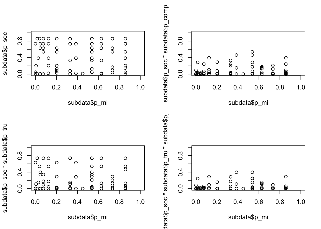 ## Wahrscheinlichkeiten nach der Empirischen Ankerpunkten
library(QCA)

fc=1  #First column
lc=18 #Last column

for(i in fc:lc) {

a=as.numeric(quantile(subdata[,i], probs = 0.05))
b=mean(subdata[,i])
c=as.numeric(quantile(subdata[,i], probs = 0.95))

subdata[paste0(colnames(subdata[i]),"_cbr") ] <- calibrate(subdata[,i], type = "fuzzy",method ="direct", c(a,b,c))
}

head(subdata)
## x141 x142 x143 x144 x145 x146 x228 x229 x231 x242 x238 x239 x234 x235 x236
## 33 3 3 3 4 4 3 5 5 4 4 4 4 4 5 5
## 35 3 2 2 4 4 4 4 2 1 2 3 2 3 2 3
## 36 1 1 2 4 4 3 3 3 2 3 1 3 3 3 3
## 92 5 5 5 3 5 1 5 5 1 3 4 3 3 3 3
## 94 5 4 4 2 4 4 4 4 5 3 3 4 4 3 3
## 108 4 4 4 4 4 3 5 4 5 4 4 5 4 4 4
## x114 mission darwin soc x141_cbr x142_cbr x143_cbr x144_cbr
## 33 1 9 11 14 0.219163871 0.221145827 0.2458917 0.7705090
## 35 1 7 12 7 0.219163871 0.050000000 0.0500000 0.7705090
## 36 1 4 11 8 0.009772791 0.009661705 0.0500000 0.7705090
## 92 1 15 9 11 0.950000000 0.950000000 0.9500000 0.4048257
## 94 1 13 10 13 0.950000000 0.644408486 0.6940924 0.1591029
## 108 1 12 11 14 0.639163588 0.644408486 0.6940924 0.7705090
## x145_cbr x146_cbr x228_cbr x229_cbr x231_cbr p_mi p_da
## 33 0.6337815 0.4743443 0.9500000 0.9500000 0.6593581 0.1250000000 0.3308053
## 35 0.6337815 0.8048694 0.5173133 0.1428689 0.0500000 0.0174108057 0.5381504
## 36 0.6337815 0.4743443 0.1893460 0.3454980 0.1349050 0.0004665137 0.3308053
## 92 0.9500000 0.0500000 0.9500000 0.9500000 0.0500000 0.8573750000 0.0237500
## 94 0.6337815 0.8048694 0.5173133 0.7125638 0.9500000 0.6285300868 0.1234602
## 108 0.6337815 0.4743443 0.9500000 0.7125638 0.9500000 0.5381504397 0.3308053
## p_soc x242_cbr x238_cbr x239_cbr x234_cbr x235_cbr x236_cbr
## 33 0.734088539 0.9500000 0.7590476 0.7768316 0.6545020 0.9500000 0.9500000
## 35 0.007589194 0.2982492 0.3891992 0.1618536 0.2252326 0.0500000 0.2385616
## 36 0.046651374 0.7489484 0.0500000 0.4147017 0.2252326 0.2741706 0.2385616
## 92 0.045125000 0.7489484 0.7590476 0.4147017 0.2252326 0.2741706 0.2385616
## 94 0.628530087 0.7489484 0.3891992 0.7768316 0.6545020 0.2741706 0.2385616
## 108 0.734088539 0.9500000 0.7590476 0.9500000 0.6545020 0.7289559 0.6818744
## p_comp p_tru x114_cbr mission_cbr darwin_cbr
## 33 0.53815044 0.73408854 NaN 0.22380450 0.6616584
## 35 0.01741081 0.04665137 NaN 0.08191543 0.8107274
## 36 0.01250000 0.12500000 NaN 0.01512660 0.6616584
## 92 0.20334863 0.12500000 NaN 0.95000000 0.3641151
## 94 0.20334863 0.20334863 NaN 0.80635514 0.4824005
## 108 0.62853009 0.53815044 NaN 0.66094944 0.6616584par(mfrow=c(2,2))
plot (subdata$p_da,subdata$p_soc, xlim=c(0,1), ylim=c(0,1))
plot (subdata$p_mi,subdata$p_soc, xlim=c(0,1), ylim=c(0,1))
plot (subdata$p_da*subdata$p_mi,subdata$p_soc, xlim=c(0,1), ylim=c(0,1))
plot ((1-subdata$p_da)*(1-subdata$p_mi),subdata$p_soc, xlim=c(0,1), ylim=c(0,1))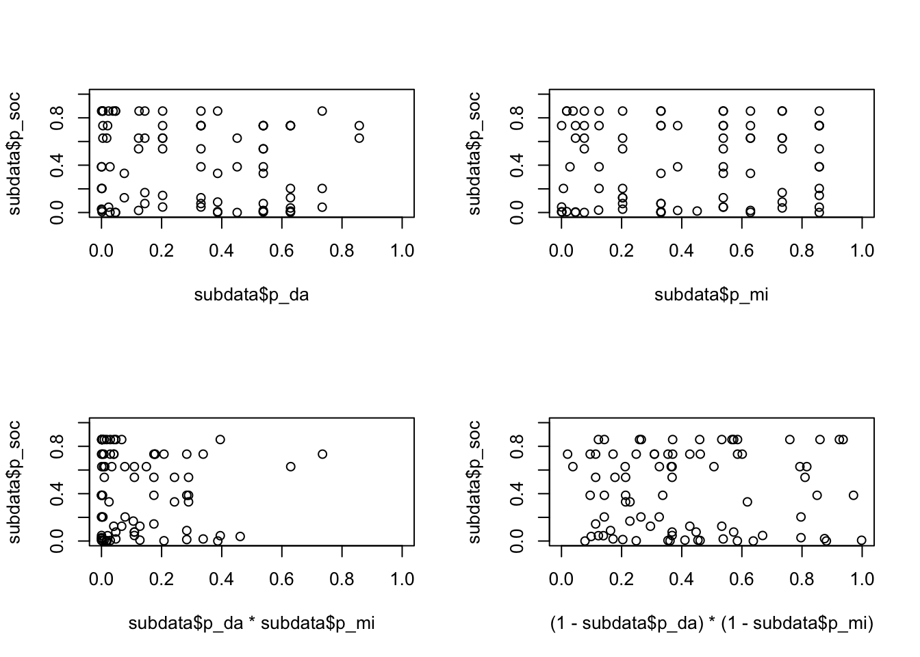
par(mfrow=c(3,3))

plot (subdata$p_da,subdata$p_soc, xlim=c(0,1), ylim=c(0,1))
plot (subdata$p_comp,subdata$p_soc, xlim=c(0,1),ylim=c(0,1))
plot (subdata$p_tru,subdata$p_soc, xlim=c(0,1),ylim=c(0,1))

plot (subdata$p_da*subdata$p_comp,subdata$p_soc, xlim=c(0,1),ylim=c(0,1))
plot (subdata$p_comp*subdata$p_tru,subdata$p_soc, xlim=c(0,1),ylim=c(0,1))
plot (subdata$p_da*subdata$p_tru,subdata$p_soc, xlim=c(0,1),ylim=c(0,1))

plot (subdata$p_da*subdata$p_comp*subdata$p_tru,subdata$p_soc, xlim=c(0,1),ylim=c(0,1))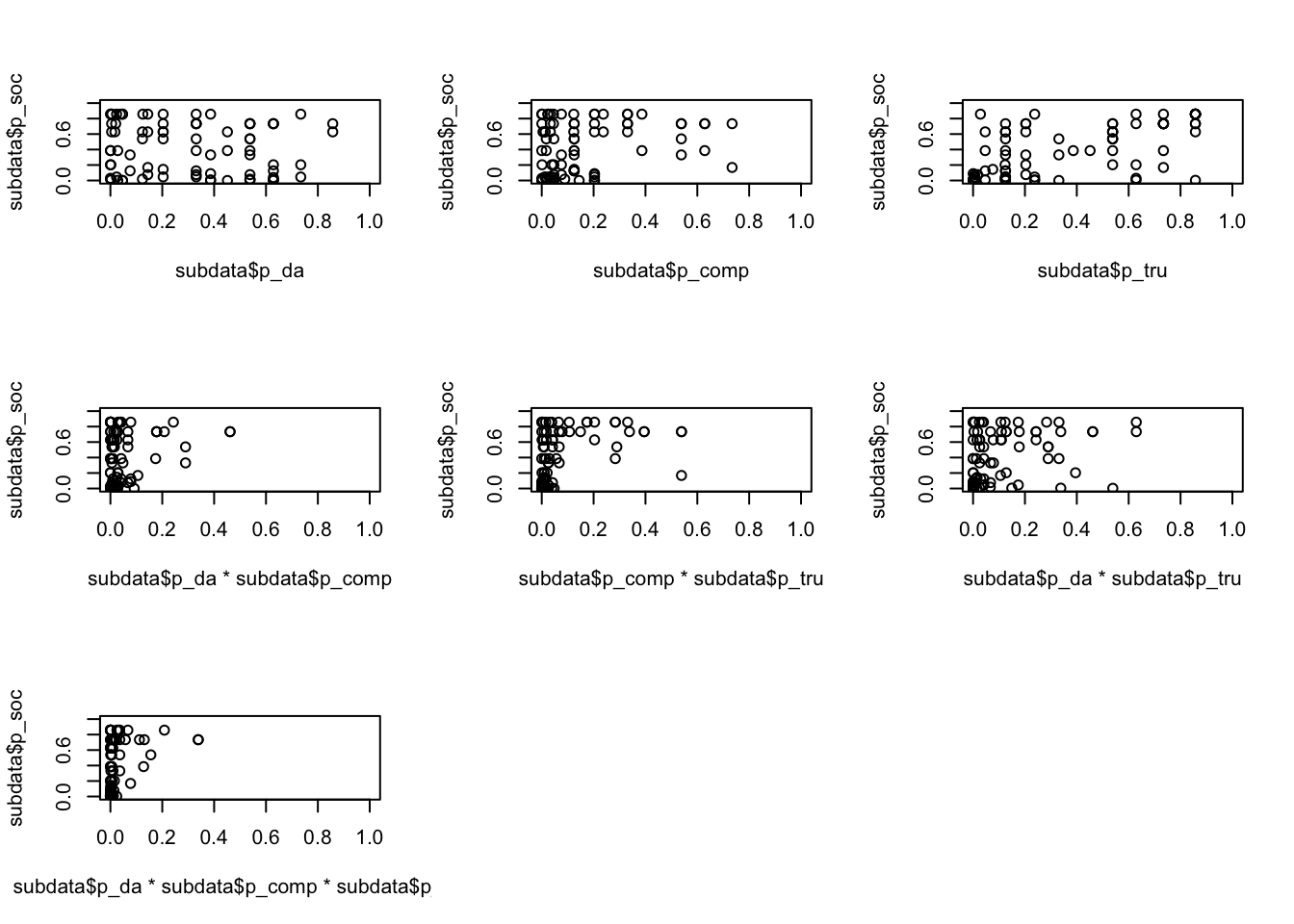
par(mfrow=c(3,3))

plot (subdata$p_mi,subdata$p_soc, xlim=c(0,1), ylim=c(0,1))
plot (subdata$p_comp,subdata$p_soc, xlim=c(0,1),ylim=c(0,1))
plot (subdata$p_tru,subdata$p_soc, xlim=c(0,1),ylim=c(0,1))

plot (subdata$p_mi*subdata$p_comp,subdata$p_soc, xlim=c(0,1),ylim=c(0,1))
plot (subdata$p_comp*subdata$p_tru,subdata$p_soc, xlim=c(0,1),ylim=c(0,1))
plot (subdata$p_mi*subdata$p_tru,subdata$p_soc, xlim=c(0,1),ylim=c(0,1))

plot (subdata$p_mi*subdata$p_comp*subdata$p_tru,subdata$p_soc, xlim=c(0,1),ylim=c(0,1))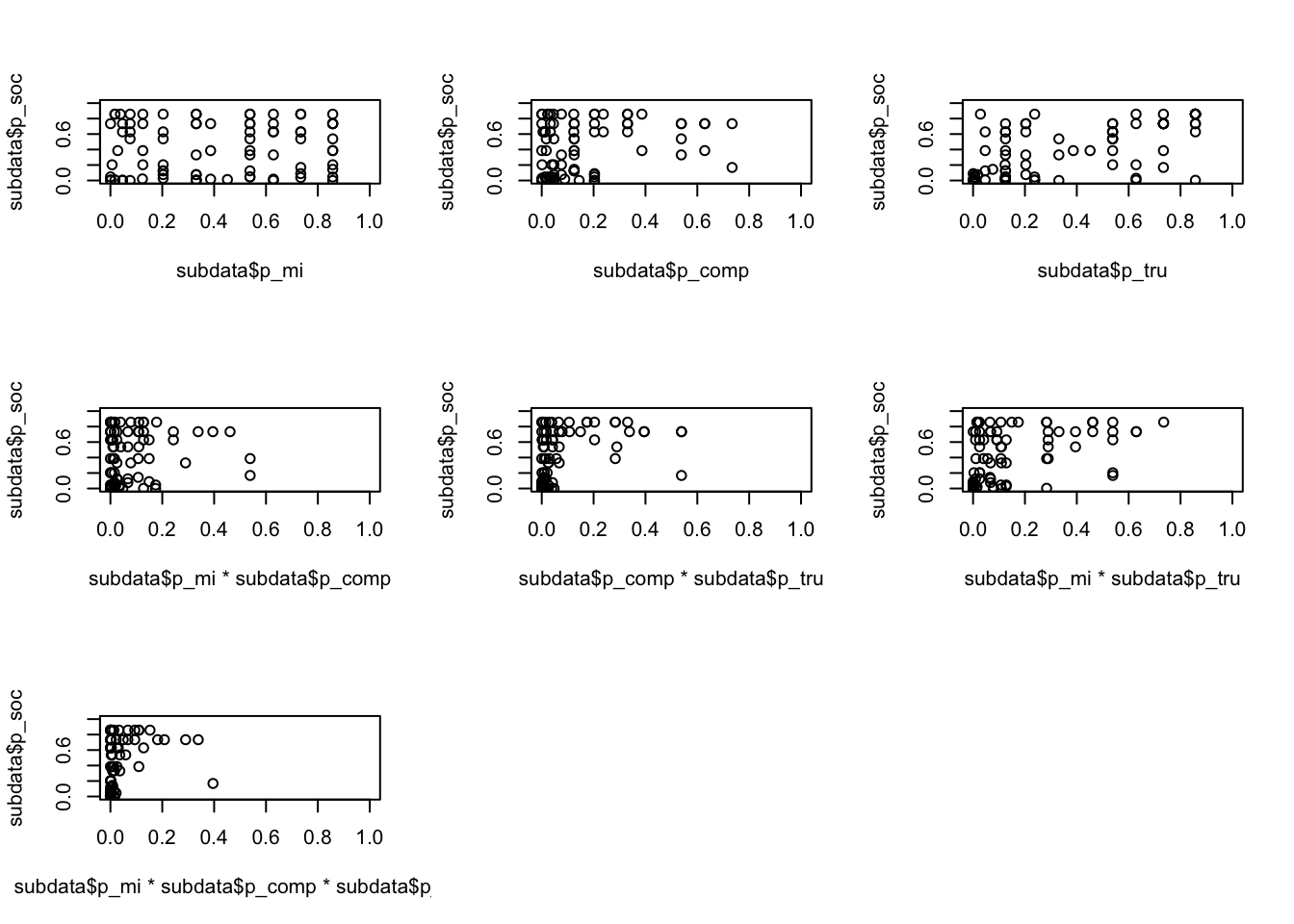
par(mfrow=c(2,2))

plot (subdata$p_da,subdata$p_soc, xlim=c(0,1), ylim=c(0,1))
plot (subdata$p_da,subdata$p_soc*subdata$p_comp, xlim=c(0,1),ylim=c(0,1))
plot (subdata$p_da,subdata$p_soc*subdata$p_tru, xlim=c(0,1),ylim=c(0,1))
plot (subdata$p_da,subdata$p_soc*subdata$p_tru*subdata$p_comp, xlim=c(0,1),ylim=c(0,1))
par(mfrow=c(2,2))

plot (subdata$p_mi,subdata$p_soc, xlim=c(0,1), ylim=c(0,1))
plot (subdata$p_mi,subdata$p_soc*subdata$p_comp, xlim=c(0,1),ylim=c(0,1))
plot (subdata$p_mi,subdata$p_soc*subdata$p_tru, xlim=c(0,1),ylim=c(0,1))
plot (subdata$p_mi,subdata$p_soc*subdata$p_tru*subdata$p_comp, xlim=c(0,1),ylim=c(0,1))