Chapter 4 Endogeneity simulation
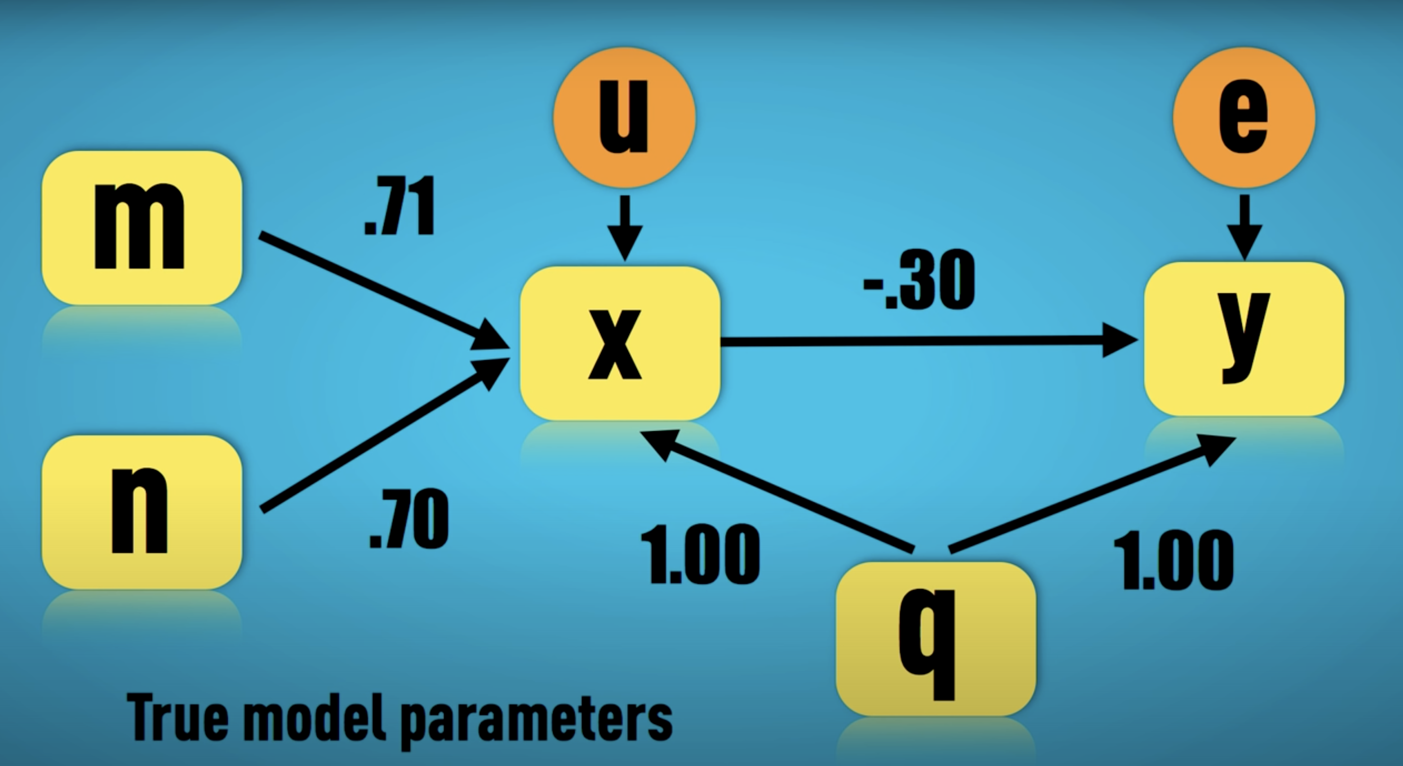
Am Anfang dieser Ausführungen steht Datensatz von Antonakis (2011), dessen Zusammenhänge bekannt, uns aber noch verborgen sind. Darin sind zwei Größen X und Y gegeben, deren Bedeutung wir hier untersuchen wollen.
plot (data$x, data$y)
cov (data$x, data$y)## [1] 0.09830745Der Plot weist auf ein unsystematischen Zusammenhang zwischen den Werten in X und den Werten in Y hin. Eine Korrelation in Höhe von 0.098 unterstütz dieses Bild.
summary (lm(data$y~data$x))##
## Call:
## lm(formula = data$y ~ data$x)
##
## Residuals:
## Min 1Q Median 3Q Max
## -4.5318 -0.8614 0.0077 0.8715 4.6860
##
## Coefficients:
## Estimate Std. Error t value Pr(>|t|)
## (Intercept) -0.009860 0.012956 -0.761 0.447
## data$x 0.032703 0.007473 4.376 1.22e-05 ***
## ---
## Signif. codes: 0 '***' 0.001 '**' 0.01 '*' 0.05 '.' 0.1 ' ' 1
##
## Residual standard error: 1.296 on 9998 degrees of freedom
## Multiple R-squared: 0.001912, Adjusted R-squared: 0.001812
## F-statistic: 19.15 on 1 and 9998 DF, p-value: 1.219e-05summary (lm(y~x, data=data))##
## Call:
## lm(formula = y ~ x, data = data)
##
## Residuals:
## Min 1Q Median 3Q Max
## -4.5318 -0.8614 0.0077 0.8715 4.6860
##
## Coefficients:
## Estimate Std. Error t value Pr(>|t|)
## (Intercept) -0.009860 0.012956 -0.761 0.447
## x 0.032703 0.007473 4.376 1.22e-05 ***
## ---
## Signif. codes: 0 '***' 0.001 '**' 0.01 '*' 0.05 '.' 0.1 ' ' 1
##
## Residual standard error: 1.296 on 9998 degrees of freedom
## Multiple R-squared: 0.001912, Adjusted R-squared: 0.001812
## F-statistic: 19.15 on 1 and 9998 DF, p-value: 1.219e-05summary (lm(y~x+q, data=data))##
## Call:
## lm(formula = y ~ x + q, data = data)
##
## Residuals:
## Min 1Q Median 3Q Max
## -3.8656 -0.6954 -0.0033 0.6841 3.4236
##
## Coefficients:
## Estimate Std. Error t value Pr(>|t|)
## (Intercept) -0.004879 0.010040 -0.486 0.627
## x -0.303346 0.007107 -42.680 <2e-16 ***
## q 1.003060 0.012299 81.554 <2e-16 ***
## ---
## Signif. codes: 0 '***' 0.001 '**' 0.01 '*' 0.05 '.' 0.1 ' ' 1
##
## Residual standard error: 1.004 on 9997 degrees of freedom
## Multiple R-squared: 0.4007, Adjusted R-squared: 0.4005
## F-statistic: 3342 on 2 and 9997 DF, p-value: < 2.2e-16library (NCA)##
## Please cite the NCA package as:
##
## Dul, J. 2022.
## Necessary Condition Analysis.
## R Package Version 3.2.1.
## URL: https://cran.r-project.org/web/packages/NCA/
##
## This package is based on:
## Dul, J. (2016) "Necessary Condition Analysis (NCA):
## Logic and Methodology of 'Necessary but Not Sufficient' Causality."
## Organizational Research Methods 19(1), 10-52.
## https://journals.sagepub.com/doi/full/10.1177/1094428115584005
## and
## Dul, J. (2020) "Conducting Necessary Condition Analysis"
## SAGE Publications, ISBN: 9781526460141
## https://uk.sagepub.com/en-gb/eur/conducting-necessary-condition-
## analysis-for-business-and-management-students/book262898
## and
## Dul, J., van der Laan, E., & Kuik, R. (2020).
## A statistical significance test for Necessary Condition Analysis."
## Organizational Research Methods, 23(2), 385-395.
## https://journals.sagepub.com/doi/10.1177/1094428118795272
##
## A BibTeX entry is provided by:
## citation('NCA')
##
## A quick start guide can be found here:
## https://repub.eur.nl/pub/78323/
## or
## https://papers.ssrn.com/sol3/papers.cfm?abstract_id=2624981
##
## For general information about NCA see :
## https://www.erim.nl/ncanca(data,c("x","q"),"y",ceilings=c("ols","ce_fdh", "cr_fdh", "ce_vrs"))##
## --------------------------------------------------------------------------------## Effect size(s):## ce_fdh cr_fdh ce_vrs
## x 0.120 0.115 0.095
## q 0.208 0.209 0.179
## --------------------------------------------------------------------------------#CE-FDH (step function)
#CR-FDH (straight line).
#CE-VRS
#OLS
model <- nca_analysis(data,c("x","q"),"y",ceilings=c("ols","ce_fdh", "cr_fdh", "ce_vrs"),test.rep=1000)## Do test for : ce_fdh - x
Done test for : ce_fdh - x
## Do test for : cr_fdh - x
Done test for : cr_fdh - x
## Do test for : ce_vrs - x
Done test for : ce_vrs - x
## Do test for : ce_fdh - q
Done test for : ce_fdh - q
## Do test for : cr_fdh - q
Done test for : cr_fdh - q
## Do test for : ce_vrs - q
Done test for : ce_vrs - qmodel##
## --------------------------------------------------------------------------------## Effect size(s):## ce_fdh p cr_fdh p ce_vrs p
## x 0.120 0.023 0.115 0.055 0.095 0.028
## q 0.208 0.001 0.209 0.001 0.179 0.001
## --------------------------------------------------------------------------------summary (model)##
## --------------------------------------------------------------------------------## NCA Parameters : x - y## --------------------------------------------------------------------------------
##
## Number of observations 10000
## Scope 131.841
## Xmin -7.134
## Xmax 6.950
## Ymin -4.621
## Ymax 4.739
##
## ce_fdh cr_fdh ce_vrs
## Ceiling zone 15.805 15.169 12.473
## Effect size 0.120 0.115 0.095
## # above 0 15 0
## c-accuracy 100% 99.8% 100%
## Fit 100% 96.0% 78.9%
## p-value 0.023 0.055 0.028
## p-accuracy 0.009 0.014 0.010
##
## Slope 0.471
## Intercept 4.318
## Abs. ineff. 96.172 101.504 96.172
## Rel. ineff. 72.945 76.990 72.945
## Condition ineff. 32.208 42.990 32.208
## Outcome ineff. 60.092 59.638 60.092
##
##
## --------------------------------------------------------------------------------
## NCA Parameters : q - y## --------------------------------------------------------------------------------
##
## Number of observations 10000
## Scope 70.002
## Xmin -3.668
## Xmax 3.810
## Ymin -4.621
## Ymax 4.739
##
## ce_fdh cr_fdh ce_vrs
## Ceiling zone 14.588 14.644 12.525
## Effect size 0.208 0.209 0.179
## # above 0 33 0
## c-accuracy 100% 99.7% 100%
## Fit 100% 99.6% 85.9%
## p-value 0.000 0.000 0.000
## p-accuracy 0.002 0.002 0.002
##
## Slope 1.018
## Intercept 3.014
## Abs. ineff. 24.544 40.715 24.544
## Rel. ineff. 35.062 58.162 35.062
## Condition ineff. 9.788 28.288 9.788
## Outcome ineff. 28.016 41.659 28.016References
Antonakis, J. (2011). Endogeneity: An inconvenient truth (full version). Web Page,. Verfügbar unter: https://www.youtube.com/watch?v=dLuTjoYmfXs&t=111s