Chapter 3 Interaktion zwischen Ursachen
3.1 Positive Interaktion
In der kovarianzbasierten Perspektive spricht man von Interaktion, wenn der Produktterm zweier Variablen (X und Z) eine Kovarianz mit einer dritten Variable (Y) aufweist (vgl. z.B. Baron & Kenny (1986)).
Formal ausgedrückt: \(cov(XZ; Y)\)
Im folgenden wird dies veranschaulicht. Zunächst werden Werte für X und Z in einem Sample von n= 250 generiert. X und Z sind voneinander unabhängige Zufallszahlen aus dem Bereich zwischen 1 und 5.
set.seed(1899)

n = 250 #Samplegröße
lower = 1 # untere Grenze
upper = 5 # obere Grenze

x = runif(n,lower,upper)
z = runif(n,lower,upper)

plot (x,z)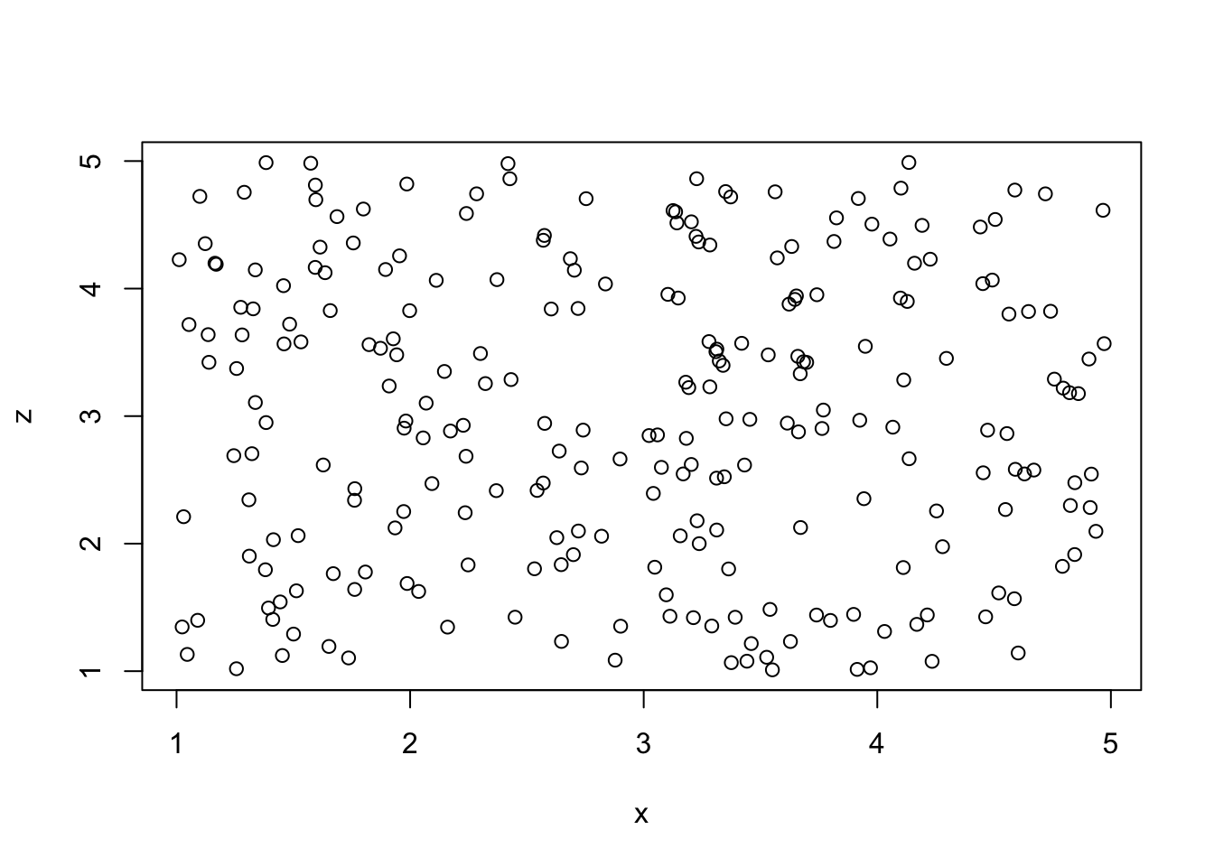
Im nächsten Schritt wird ein Produktterm (x_z) aus den mittelwert-zentrierten Variablen X und Z berechnet.
x_z = (x-mean(x))* (z-mean(z))Anschließend wird die dritte Variable (Y) als Ergebnis von X, Z, ihrer Interaktion X_Z und einem zusätzlichen Zufallsterm generiert.
y = 0.5*x + 0.5*z + 0.5*x_z + runif(n,lower,upper)Aus den drei folgenden Plots ist ersichtlich, dass sowohl X als auch Z und die Interaktion X_Z notwendige Bedingungen (Nessesary conditions) für Y darstellen. Im Sinne der Mengenlogik handelt es sich bei den beiden Variablen X und Z sowie bei ihrer Interaktion Supersets (Obermengen) von Y. In der Sprache der Logik folgt:
\(X \leftarrow Y\)
\(Z \leftarrow Y\)
(\(X*Y \leftarrow Y\))
par(mfrow=c(1,3))

plot(x,y)
abline(lm(y~x))

plot(z,y)
abline(lm(y~z))

plot(x_z,y)
abline(lm(y~x_z))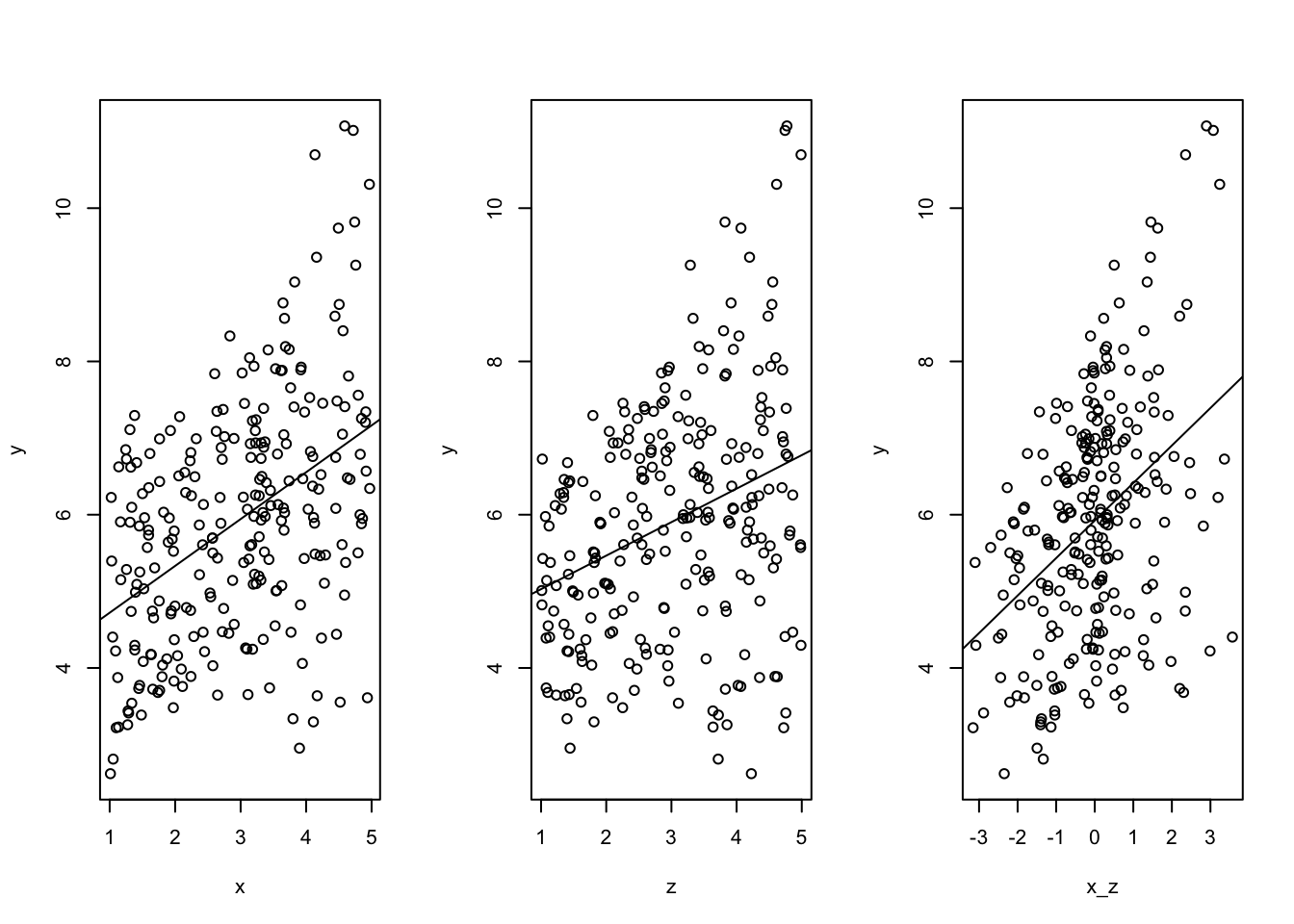
Die dargestellten Regressionsgeraden sind signifikant und werden auch in einem multivariaten Regressionsmodell bestätigt.
summary (lm(y~x+z+(x_z)))##
## Call:
## lm(formula = y ~ x + z + (x_z))
##
## Residuals:
## Min 1Q Median 3Q Max
## -2.18475 -0.98477 0.05851 0.92919 2.03907
##
## Coefficients:
## Estimate Std. Error t value Pr(>|t|)
## (Intercept) 2.66552 0.27720 9.616 < 2e-16 ***
## x 0.61706 0.06328 9.751 < 2e-16 ***
## z 0.47889 0.06242 7.673 3.94e-13 ***
## x_z 0.50409 0.05525 9.124 < 2e-16 ***
## ---
## Signif. codes: 0 '***' 0.001 '**' 0.01 '*' 0.05 '.' 0.1 ' ' 1
##
## Residual standard error: 1.135 on 246 degrees of freedom
## Multiple R-squared: 0.4823, Adjusted R-squared: 0.476
## F-statistic: 76.39 on 3 and 246 DF, p-value: < 2.2e-16Das Ziel der Interaktionsanalyse ist der Nachweis bedeutsamer Interaktion und die Prognose von Ergebnissen durch die interagierenden Variablen. Es kann z.B. interessant sein, wie der Zusammenhang von X und Y auf verschiedenen Niveau von Z verändert. Im folgenden werden die Datenpunkte durch unterschiedliche Blautöne dargestellt.
data <-data.frame(cbind(x, z, y))
data <- subset(data, (z>=1.7 & z<=1.9  | z>=4.1 & z<=4.3))

library(ggplot2)
ggplot (data, aes(x=x, y=y)) +
  geom_point(aes(color= z))+ theme_minimal()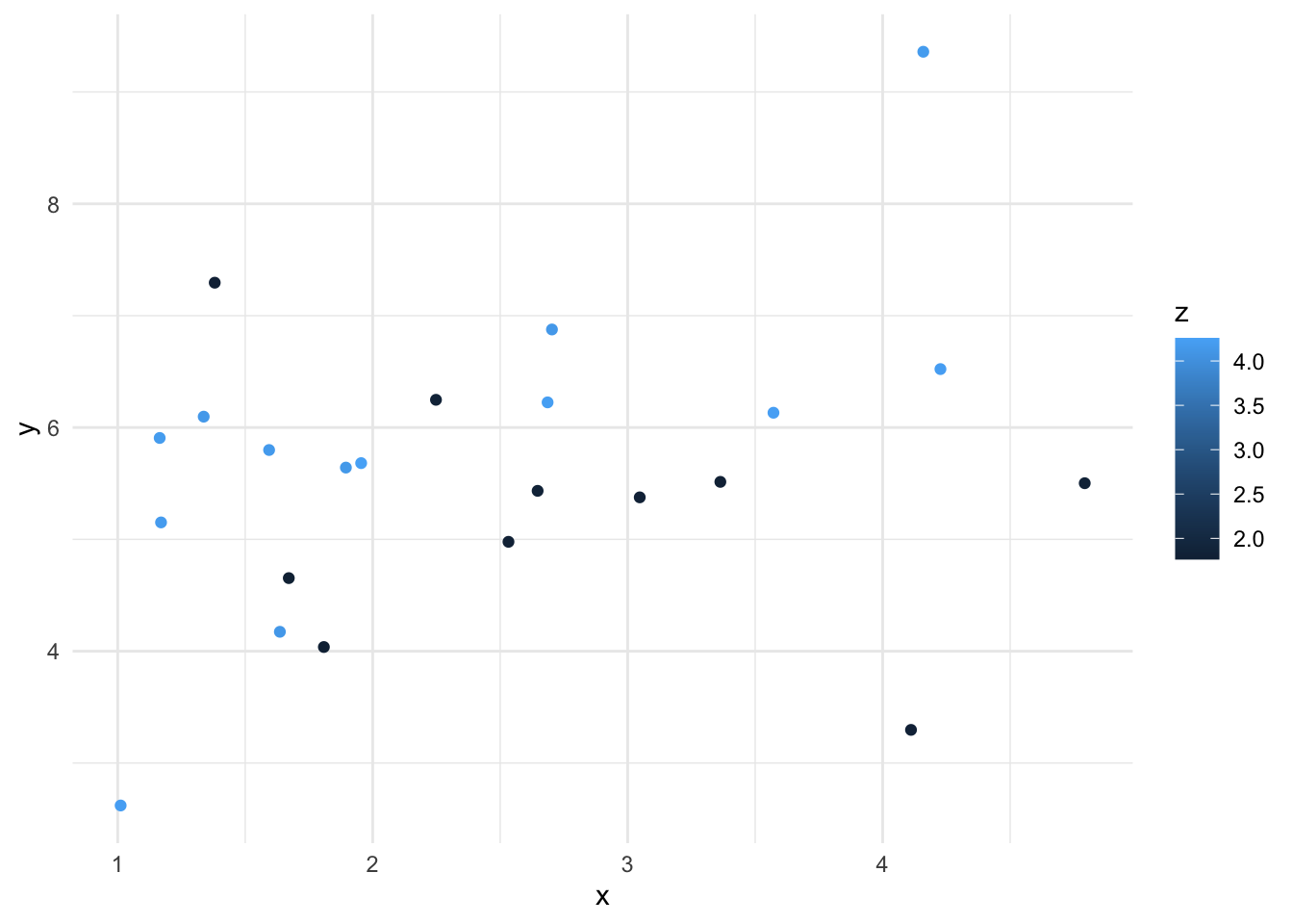
Hier lässt sich nur erahnen, was im nächsten Plot deutlicher wird. Links, bei gering ausgeprägten z, zeigt sich ein geringer Anstieg in Y durch steigende X. Rechts, bei hoch ausgeprägten z, ist der Anstieg deutlich stärker ausgeprägt.
par(mfrow=c(1,2))

data <-data.frame(cbind(x, z, y))
data <- subset(data, (data$z>=1.7 & data$z<=1.9))

plot(data$x,data$y, main="1.7< z < 1.9", xlim=c(1,6), ylim=c(1,10), xlab="real x-values", ylab="real y-values")
abline(lm(data$y~data$x))

data <-data.frame(cbind(x, z, y))
data <- subset(data, (data$z>=4.1 & data$z<=4.3))

plot(data$x,data$y, main="4.1< z < 4.3", xlim=c(1,6), ylim=c(1,10), xlab="real x-values", ylab="real y-values")
abline(lm(data$y~data$x))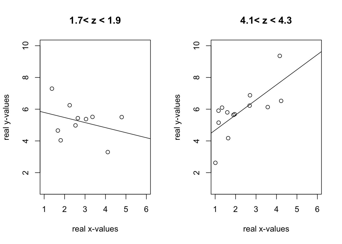
Die Plots zeigen bis hierhin die realen Werte. Im folgenden sollen diese Plots nun Werte aus den geschätzten Regressionskoeffizienten aufzeigen.
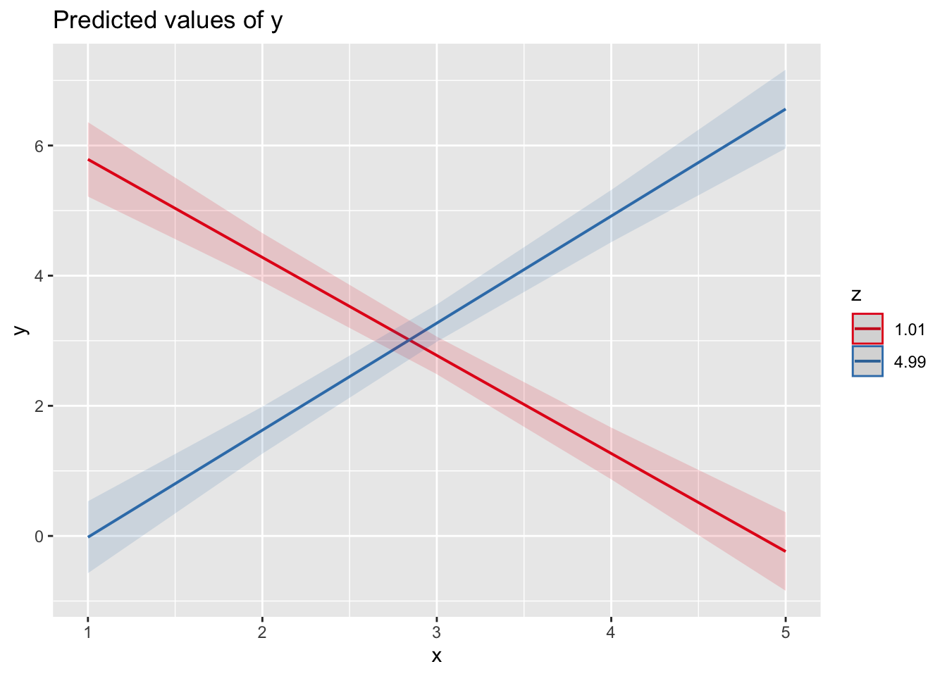
Eine mögliche Darstellung bietet das Paket Lüdecke (o. J.) . Dabei ist der Interaktionsterm in der Regressionsgleichung unzentriert in Form “x*z” einzusetzen.
summary (lm(y~x+z+(x_z)))##
## Call:
## lm(formula = y ~ x + z + (x_z))
##
## Residuals:
## Min 1Q Median 3Q Max
## -2.18475 -0.98477 0.05851 0.92919 2.03907
##
## Coefficients:
## Estimate Std. Error t value Pr(>|t|)
## (Intercept) 2.66552 0.27720 9.616 < 2e-16 ***
## x 0.61706 0.06328 9.751 < 2e-16 ***
## z 0.47889 0.06242 7.673 3.94e-13 ***
## x_z 0.50409 0.05525 9.124 < 2e-16 ***
## ---
## Signif. codes: 0 '***' 0.001 '**' 0.01 '*' 0.05 '.' 0.1 ' ' 1
##
## Residual standard error: 1.135 on 246 degrees of freedom
## Multiple R-squared: 0.4823, Adjusted R-squared: 0.476
## F-statistic: 76.39 on 3 and 246 DF, p-value: < 2.2e-16#summary (lm(scale(y)~scale(x)+scale(z)+scale(x_z)))
#install.packages("sjPlot")
library(sjPlot)
#library(sjmisc)
#library(ggplot2)
#theme_set(theme_sjplot())
fit <- lm(y~x+z+x*z)
par(mfrow=c(1,2))
plot_model(fit, type='int', terms=c("x","z","x*z"))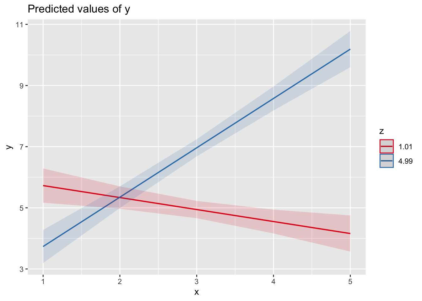
Am Rande sei hier aufgezeigt, dass diese Form nicht in gleicher Weise zum richtigen Ergebnis in der Regression führt.
summary (lm(y~x+z+x*z))##
## Call:
## lm(formula = y ~ x + z + x * z)
##
## Residuals:
## Min 1Q Median 3Q Max
## -2.18475 -0.98477 0.05851 0.92919 2.03907
##
## Coefficients:
## Estimate Std. Error t value Pr(>|t|)
## (Intercept) 7.13486 0.55812 12.784 < 2e-16 ***
## x -0.90125 0.17856 -5.047 8.72e-07 ***
## z -1.00496 0.17145 -5.862 1.47e-08 ***
## x:z 0.50409 0.05525 9.124 < 2e-16 ***
## ---
## Signif. codes: 0 '***' 0.001 '**' 0.01 '*' 0.05 '.' 0.1 ' ' 1
##
## Residual standard error: 1.135 on 246 degrees of freedom
## Multiple R-squared: 0.4823, Adjusted R-squared: 0.476
## F-statistic: 76.39 on 3 and 246 DF, p-value: < 2.2e-16Während der Regressionskoeffizient des Interaktionsterms das identische Ergebnis aufzeigt, weisen die Regressionskoeffizienten für X und Z negative Vorzeichen auf.
Die näherungsweise besseren Schätzungen für alle Regressionskoeffizienten werden ermittelt, wenn der mittelwertzentrierte Produktterm in die Regressionsgleichung eingesetzt wird.
summary (lm(y~x+z+(x_z)))##
## Call:
## lm(formula = y ~ x + z + (x_z))
##
## Residuals:
## Min 1Q Median 3Q Max
## -2.18475 -0.98477 0.05851 0.92919 2.03907
##
## Coefficients:
## Estimate Std. Error t value Pr(>|t|)
## (Intercept) 2.66552 0.27720 9.616 < 2e-16 ***
## x 0.61706 0.06328 9.751 < 2e-16 ***
## z 0.47889 0.06242 7.673 3.94e-13 ***
## x_z 0.50409 0.05525 9.124 < 2e-16 ***
## ---
## Signif. codes: 0 '***' 0.001 '**' 0.01 '*' 0.05 '.' 0.1 ' ' 1
##
## Residual standard error: 1.135 on 246 degrees of freedom
## Multiple R-squared: 0.4823, Adjusted R-squared: 0.476
## F-statistic: 76.39 on 3 and 246 DF, p-value: < 2.2e-16Dawson (2014) erklärt, “it is crucially important that the interaction term is calculated from the same form of the main variables that are entered into the regression; so if X and Z are centered to form new variables Xc and Zc, then the term XZ is calculated by multiplying Xc and Zc together (this interaction term is then left as it is, rather than itself being centered). The dependent variable, Y, is left in its raw form. An ordinary regression analysis can then be used with Y as the dependent variable, and Xc, Zc, and XZ as the independent variables.”
In seiner Interpretation von Interaktionseffekten schreibt er:_“It is recommended that the independent variable and moderator are centred before calculation of the product term, although this is not essential. The product term should be significant in the regression equation in order for the interaction to be interpretable”(http://www.jeremydawson.co.uk/slopes.htm).
In der aktuellen Excel-Version zum Plotten von Interaktionen “2-way_linear_interactions.xls” berücksichtigt er die Mittelwerte und Standardabweichungen der unabhängigen Variable und des Moderators, wenn er Schätzungen für die Ergebnisvariable bestimmt.
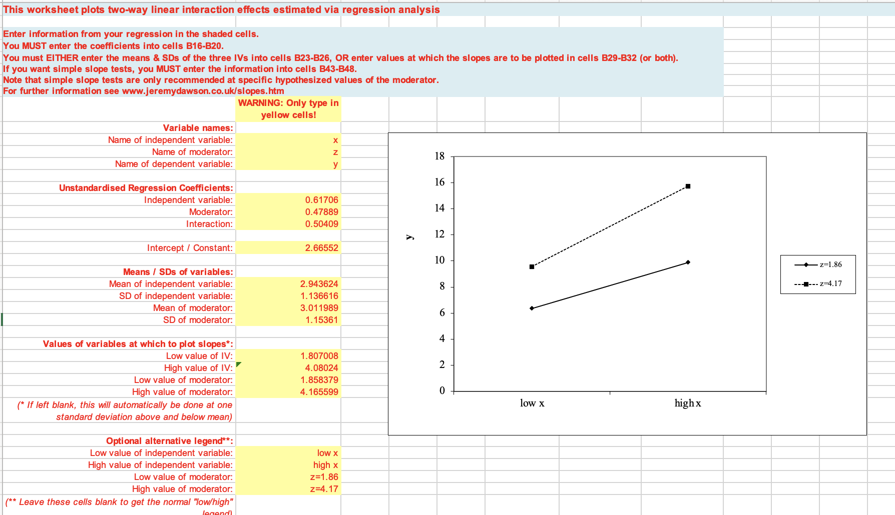
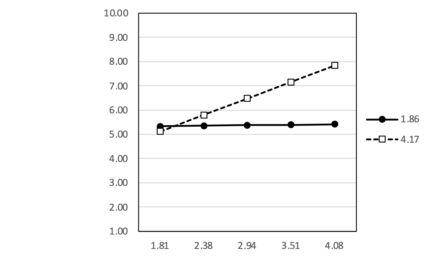
Es verwundert, dass sich die beiden Geradenbei “low x” nicht, wie in der vorherigen Abbildung, kreuzen. Das Label “low X” steht hier für einen Wert von \(mean(x)-sd(x) = 1.81\).
Die Abbildung kann aufgrund der Schätzgleichung einfach repliziert werden. Die Werte ergeben sich aus:
\[\hat{y}=0.617 \cdot x + 0.478 \cdot z + 0.504 \cdot x \cdot z\]
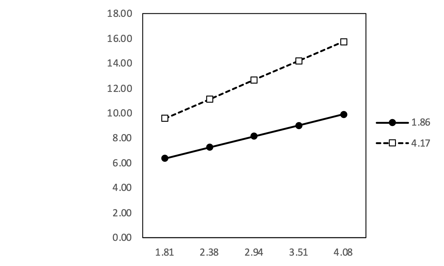
Bei genauerem Hinsehen irritieren die hoch geschätzten Werte für Y. Hier verweise ich noch einmal darauf, dass “it is crucially important that the interaction term is calculated from the same form of the main variables that are entered into the regression” Dawson (2014). Die geschätzen Werte für Y ergeben sich demnach aus:
\[\hat{y}=0.617 \cdot x + 0.478 \cdot z + 0.504 \cdot (x-mean(x) \cdot (z-mean(z))\] Hier bietet sich nun folgendes Bild:
Anders als in diesem Beispiel, in dem wir die “wahren” Zusammenhänge kennen, kann die Unwissenheit über die tatsächlichen Zusammenhänge zu vielen Missinterpretationen führen. Dies bezieht die geschätzen Koeffizienten der Regressionsgleichung ein und das Plotten der Ergebnisse
Im Sinne der Mengenlogik handelt es sich bei den beiden Variablen “X” und “Z” und ihrer Interaktion (in Form des Produkttermes) um notwendige Bedingungen (Nessesary condition).
In der Sprache der Logik folgt:
\(X \leftarrow Y\)
\(Z \leftarrow Y\)
(\(X*Z \leftarrow Y\))
##
## Please cite the NCA package as:
##
##   Dul, J. 2022.
##   Necessary Condition Analysis.
##   R Package Version 3.2.1.
##   URL: https://cran.r-project.org/web/packages/NCA/
##
## This package is based on:
##   Dul, J. (2016) "Necessary Condition Analysis (NCA):
##   Logic and Methodology of 'Necessary but Not Sufficient' Causality."
##   Organizational Research Methods 19(1), 10-52.
##   https://journals.sagepub.com/doi/full/10.1177/1094428115584005
## and
##   Dul, J. (2020) "Conducting Necessary Condition Analysis"
##   SAGE Publications, ISBN: 9781526460141
##   https://uk.sagepub.com/en-gb/eur/conducting-necessary-condition-
##   analysis-for-business-and-management-students/book262898
## and
##   Dul, J., van der Laan, E., & Kuik, R. (2020).
##   A statistical significance test for Necessary Condition Analysis."
##   Organizational Research Methods, 23(2), 385-395.
##   https://journals.sagepub.com/doi/10.1177/1094428118795272
##
## A BibTeX entry is provided by:
##   citation('NCA')
##
## A quick start guide can be found here:
##   https://repub.eur.nl/pub/78323/
##   or
##   https://papers.ssrn.com/sol3/papers.cfm?abstract_id=2624981
##
## For general information about NCA see :
##   https://www.erim.nl/nca
##
## --------------------------------------------------------------------------------## Effect size(s):## ce_fdh cr_fdh ce_vrs
## x 0.314 0.301 0.222
## z 0.320 0.309 0.244
## --------------------------------------------------------------------------------## Do test for : ce_fdh - x
Done test for : ce_fdh - x
## Do test for : cr_fdh - x
Done test for : cr_fdh - x
## Do test for : ce_vrs - x
Done test for : ce_vrs - x
## Do test for : ce_fdh - z
Done test for : ce_fdh - z
## Do test for : cr_fdh - z
Done test for : cr_fdh - z
## Do test for : ce_vrs - z
Done test for : ce_vrs - z##
## --------------------------------------------------------------------------------## Effect size(s):## ce_fdh p cr_fdh p ce_vrs p
## x 0.314 0.001 0.301 0.001 0.222 0.001
## z 0.320 0.001 0.309 0.001 0.244 0.001
## --------------------------------------------------------------------------------summary (model)##
## --------------------------------------------------------------------------------## NCA Parameters : x - y## --------------------------------------------------------------------------------
##
## Number of observations 250
## Scope 33.471
## Xmin 1.011
## Xmax 4.971
## Ymin 2.620
## Ymax 11.073
##
## ce_fdh cr_fdh ce_vrs
## Ceiling zone 10.499 10.075 7.417
## Effect size 0.314 0.301 0.222
## # above 0 16 0
## c-accuracy 100% 93.6% 100%
## Fit 100% 96.0% 70.6%
## p-value 0.000 0.000 0.000
## p-accuracy 0.002 0.002 0.002
##
## Slope 1.389
## Intercept 4.379
## Abs. ineff. 3.232 13.321 3.232
## Rel. ineff. 9.656 39.798 9.656
## Condition ineff. 9.656 3.799 9.656
## Outcome ineff. 0.000 37.421 0.000
##
##
## --------------------------------------------------------------------------------
## NCA Parameters : z - y## --------------------------------------------------------------------------------
##
## Number of observations 250
## Scope 33.628
## Xmin 1.010
## Xmax 4.989
## Ymin 2.620
## Ymax 11.073
##
## ce_fdh cr_fdh ce_vrs
## Ceiling zone 10.770 10.404 8.204
## Effect size 0.320 0.309 0.244
## # above 0 14 0
## c-accuracy 100% 94.4% 100%
## Fit 100% 96.6% 76.2%
## p-value 0.000 0.000 0.000
## p-accuracy 0.002 0.002 0.002
##
## Slope 1.337
## Intercept 4.448
## Abs. ineff. 10.820 12.819 10.820
## Rel. ineff. 32.175 38.121 32.175
## Condition ineff. 5.437 0.832 5.437
## Outcome ineff. 28.275 37.602 28.2753.2 Negative interaction
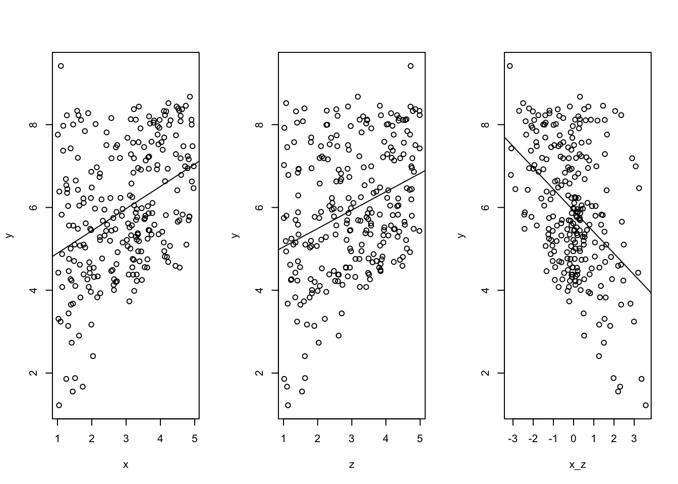
Wenn die Variablen X und Z eine negative Interaktion in Y aufweisen, stellen sich die Variablen X und Z in den einzelnen Plots als hinreichende Bedingung (Sufficiency) für Y dar.
##
## Call:
## lm(formula = y ~ x + z + x_z)
##
## Residuals:
## Min 1Q Median 3Q Max
## -1.9688 -1.0135 -0.1070 0.9948 2.1842
##
## Coefficients:
## Estimate Std. Error t value Pr(>|t|)
## (Intercept) 2.99681 0.29009 10.331 < 2e-16 ***
## x 0.55388 0.06622 8.364 4.56e-15 ***
## z 0.43083 0.06532 6.596 2.57e-10 ***
## x_z -0.50494 0.05782 -8.733 3.86e-16 ***
## ---
## Signif. codes: 0 '***' 0.001 '**' 0.01 '*' 0.05 '.' 0.1 ' ' 1
##
## Residual standard error: 1.187 on 246 degrees of freedom
## Multiple R-squared: 0.4375, Adjusted R-squared: 0.4307
## F-statistic: 63.78 on 3 and 246 DF, p-value: < 2.2e-16##
## --------------------------------------------------------------------------------## Effect size(s):## ce_fdh cr_fdh ce_vrs
## x 0.005 0.002 0.002
## z 0.097 0.117 0.053
## --------------------------------------------------------------------------------## Do test for : ce_fdh - x
Done test for : ce_fdh - x
## Do test for : cr_fdh - x
Done test for : cr_fdh - x
## Do test for : ce_vrs - x
Done test for : ce_vrs - x
## Do test for : ce_fdh - z
Done test for : ce_fdh - z
## Do test for : cr_fdh - z
Done test for : cr_fdh - z
## Do test for : ce_vrs - z
Done test for : ce_vrs - z##
## --------------------------------------------------------------------------------## Effect size(s):## ce_fdh p cr_fdh p ce_vrs p
## x 0.005 0.975 0.002 0.977 0.002 0.975
## z 0.097 0.120 0.117 0.081 0.053 0.198
## --------------------------------------------------------------------------------##
## --------------------------------------------------------------------------------## NCA Parameters : x - y## --------------------------------------------------------------------------------
##
## Number of observations 250
## Scope 32.454
## Xmin 1.011
## Xmax 4.971
## Ymin 1.222
## Ymax 9.418
##
## ce_fdh cr_fdh ce_vrs
## Ceiling zone 0.147 0.073 0.073
## Effect size 0.005 0.002 0.002
## # above 0 0 0
## c-accuracy 100% 100% 100%
## Fit 100% 50.0% 50%
## p-value 0.975 0.977 0.975
## p-accuracy 0.010 0.009 0.010
##
## Slope 18.782
## Intercept -11.237
## Abs. ineff. 32.308 32.308 32.308
## Rel. ineff. 99.549 99.549 99.549
## Condition ineff. 97.770 97.770 97.770
## Outcome ineff. 79.760 79.760 79.760
##
##
## --------------------------------------------------------------------------------
## NCA Parameters : z - y## --------------------------------------------------------------------------------
##
## Number of observations 250
## Scope 32.607
## Xmin 1.010
## Xmax 4.989
## Ymin 1.222
## Ymax 9.418
##
## ce_fdh cr_fdh ce_vrs
## Ceiling zone 3.154 3.800 1.733
## Effect size 0.097 0.117 0.053
## # above 0 12 0
## c-accuracy 100% 95.2% 100%
## Fit 100% 79.5% 54.9%
## p-value 0.120 0.081 0.198
## p-accuracy 0.020 0.017 0.025
##
## Slope 0.593
## Intercept 6.695
## Abs. ineff. 18.971 25.006 18.971
## Rel. ineff. 58.182 76.690 58.182
## Condition ineff. 6.682 10.034 6.682
## Outcome ineff. 55.187 74.090 55.187Wenn zwei Variablen über einen positiven Effekt hinaus auch eine positive Interaktion aufweisen, stellen sie sich als notwendige Bedingungen (nessesary conditions) dar. Werden die positiven Effekte von X und Z von einem negativen Interaktionsterm begleitet, stellen sich X und Z als hinreichende (sufficiency) Bedingungen dar.
3.3 Nur-Interaktion
Gelegentlich wird ein signifikanter Produktterme (X_Z) vorgefunden, der von insignifikanten Koeffizienten bei X und Z begleitet wird. Es kann angenommen werden, dass die Werte insignifikanter Koeffizienten (für X und Z) gleich Null sind. Anders formuliert, da der Signifikanztest überprüft, ob die Regressionskoeffizienten signifikant von Null abweichen, wird bei fehlender Signifikanz davon ausgegangen werden, dass die Regressionskoeffizienten gleich Null sind.
Im folgenden wird aufgezeigt, welche Konsequenzen dies hat und wie das gemeinsame Wirken solcher Variablen interpretiert werden kann.
Beginnen wir mit einem positiven Interaktionsterm: die Plots zeigen unsystematische Zusammenhänge für X und Z auf. Nur der Produktterm X_Z weist einen positiven Zusammenhang mit Y auf.
y = 0*x + 0*z + 0.75*x_z + runif(n,lower,upper)

par(mfrow=c(1,3))

plot(x,y)
abline(lm(y~x))

plot(z,y)
abline(lm(y~z))

plot(x_z,y)
abline(lm(y~x_z))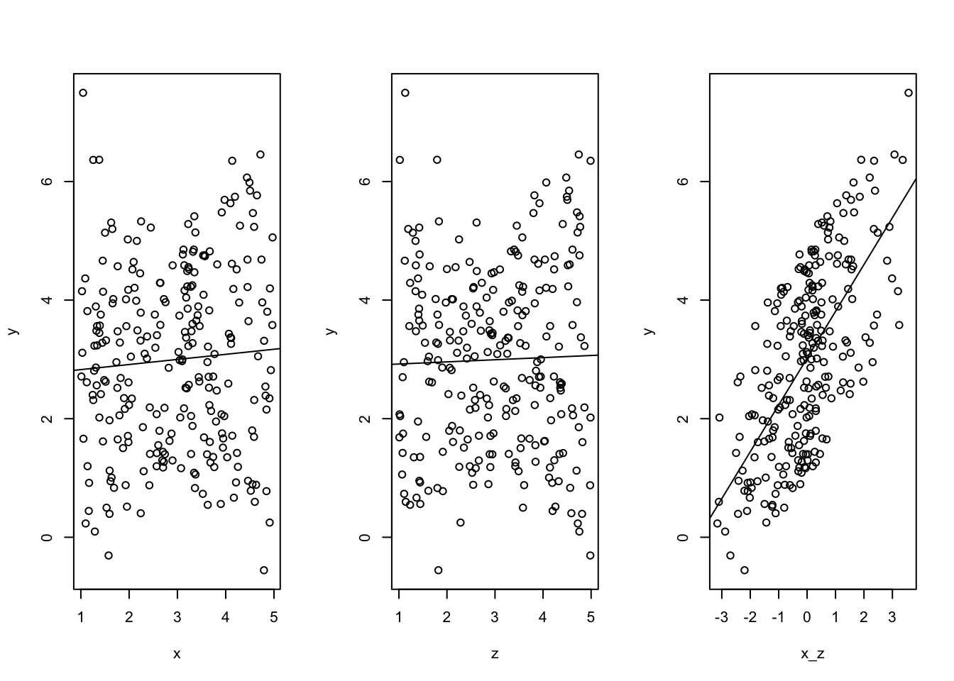
summary(lm(y~x+z+x_z))##
## Call:
## lm(formula = y ~ x + z + x_z)
##
## Residuals:
## Min 1Q Median 3Q Max
## -2.29394 -0.97673 0.00896 0.97172 2.07473
##
## Coefficients:
## Estimate Std. Error t value Pr(>|t|)
## (Intercept) 2.54695 0.28312 8.996 <2e-16 ***
## x 0.07870 0.06463 1.218 0.225
## z 0.08005 0.06375 1.256 0.210
## x_z 0.79194 0.05643 14.034 <2e-16 ***
## ---
## Signif. codes: 0 '***' 0.001 '**' 0.01 '*' 0.05 '.' 0.1 ' ' 1
##
## Residual standard error: 1.159 on 246 degrees of freedom
## Multiple R-squared: 0.4473, Adjusted R-squared: 0.4406
## F-statistic: 66.36 on 3 and 246 DF, p-value: < 2.2e-16fit <- lm(y~x+z+x*z)
plot_model(fit, type='int', terms=c("x","z","x*z"))## Warning: Could not recover model data from environment. Please make sure your
## data is available in your workspace.
## Trying to retrieve data from the model frame now.